How do SVMs and least-squares regression behave in high-dimensional settings? (NeurIPS 2021 paper with Navid and Daniel)
[technical research neural-net learning-theory Hello, it’s been a few weeks since I finished my candidacy exam, and I’m looking forward to getting back to blogging on a regular basis. I’m planning on focusing primarily on summarizing others’ works and discussing what I find interesting in the literature, but I periodically want to share my own papers and explain them less formally. I did this a few months ago for first grad student paper on the approximation capabilities of depth-2 random-bottom-layer neural networks HSSV21.
This post does the same for my second paper, which is on support vector machines (SVMs) and ordinary least-squares regression (OLS) in high-dimensional settings. I wrote this paper in collaboration with Navid Ardeshir, another third-year PhD student at Columbia studying Statistics, and our advisor, Daniel Hsu. It will appears at NeurIPS 2021 this week: a talk recorded by Navid is here, our paper reviews are here, and our poster will be virtually presented on Thursday 12/9 between 8:30am and 10am Pacific time.
I’d love to talk with anyone about this paper, so if you have any questions, comments, or rants, please comment on this post or send me an email.
What are OLS and SVMs?
The key result of our paper is that two linear machine learning models coincide in the high-dimensional setting. That is, when the dimension \(d\) is much larger than that number of samples \(n\), the solutions of the two models on the same samples have the same parameters. This is notable because the models have different structures and appear at first-glance to incentivize different kinds of solutions. It’s also perplexing because the models do not seem to be analogous–OLS is a regression learning algorithm and SVM is a classification algorithm. We’ll briefly explain what the two models are below and what they mean in the high-dimensional setting.
Both of these models were discussed extensively in my survey on over-parameterized ML models, and I’ll periodically refer back to some of those paper summaries (and occasionally steal visuals from my past self).
OLS regression and minimum-norm interpolation
The task of ordinary least-squares (OLS) regression is simple: find the linear function (or hyperplane) that best fits some data \((x_1, y_1), \dots, (x_n, y_n) \in \mathbb{R}^d \times \mathbb{R}\). To do so, we learn the function \(x \mapsto w_{OLS}^T x\), where \(w_{OLS}\) solves the following optimization problem, minimizing the mean-squared error between training labels \(y_i\) and each prediction \(w_{OLS}^T x_i\):
\[w_{OLS} \in \arg\min_{w \in \mathbb{R}^d} \sum_{i=1}^n (y_i - w_{OLS}^T x_i)^2.\]For the “classical” learning regime, where \(d \ll n\), \(w_{OLS}\) can be explicitly computed with \(w_{OLS} = X^{\dagger} y = (X^T X)^{-1} X^T y\), where \(X = (x_1, \dots, x_n) \in \mathbb{R}^{n \times d}\) and \(y = (y_1, \dots, y_n) \in \mathbb{R}^d\) collect all of the training inputs and labels into a single matrix and vector, and where \(X^{\dagger}\) is the pseudoinverse of \(X\). In the event where \(X^T X \in \mathbb{R}^{d \times d}\) is invertible (which is typically true when \(d \ll n\), although it may not be in cases where there is a lot of redundancy in the features and the columns of \(X\) are colinear), the corresponds to the unique minimizer of the above optimization problem. Intuitively, this corresponds to choosing the linear function that will most closely approximate the labels of the samples, but one that will not likely perfectly fit the data.
As discussed in my blog posts on BHX19 and BLLT19, this works well in the under-parameterized regime, but it’s not directly obvious how one should choose the best parameter vector \(w_{OLS}\) in the over-parameterized regime \(d \gg n\), since there are many parameter vectors that result in zero training error. These papers choose the vector by considering minimum-norm interpolation as the high-dimensional analogue to OLS. This entails solving the following optimization problem, which relies on \(XX^T \in \mathbb{R}^{n \times n}\) being invertible, which is typically the case when \(d \gg n\):
\[w_{OLS} \in \arg\min_{w \in \mathbb{R}^d} \|w\|_2 \ \text{such that} \ w^T x_i = y_i \ \forall i \in [n].\]In other words, it chooses the hyperplane with the smallest weight norm (which we can think of as the “smoothest” hyperplane or the hyperplane with smallest slope) that perfectly fits the data. Conveniently, this hyperplane is also found by using the pseudo-inverse of \(X\): \(w_{OLS} = X^{\dagger} y = X^T (X X^T)^{-1} y\). As a result, we (and numerous papers that consider over-parameterized linear models) consider this minimum-norm interpolation problem to be the high-dimensional version of OLS, which allows OLS to be defined with the same psuedo-inverse solution for all choices of \(n\) and \(d\).
Notably, these other papers show that high-dimensional OLS can have good generalization under certain distributional assumptions, despite the fact that classical generalization bound approaches (like VC-dimension) suggest that models with more parameters than samples are likely to fail. These results are a big part of the inspiration for this project and motivate the study of high-dimensional linear regression.
Support vector machines
SVMs are a classification problem, rather than a regression problem, which means that a training sample \((x_i, y_i)\) can be thought of as belonging to \(\mathbb{R}^d \times \{-1, 1\}\). Instead, the goal is to learn a linear classifier of the form \(x \mapsto \text{sign}(w_{SVM}^T x)\) that decisively classifies every training sample. That is, we want it to be the case that \(w_{SVM}^T x_i\) be bounded away from zero for every \(x_i\). This follows the same motivation as the generalization bounds on boosting the margin; decisively categorizing each training sample makes it hard for the chosen function to be corrupted by the variance of the training data. It also requires the assumption that the training data are linearly separable.
This high-level goal for a classifier (called the hard-margin SVM) can be encoded as the following optimization problem, which asks that \(w_{SVM}\) be the lowest-magnitude classifier that separates the samples from the decision boundary by distance at least one:
\[w_{SVM} \in \arg\min_{w \in \mathbb{R}^d} \|w\|_2 \ \text{such that} \ y_i w^T x_i \geq 1 \ \forall i \in [n].\]By stealing an image from my past blog post, we can visualize the classifiers have maximum margin.
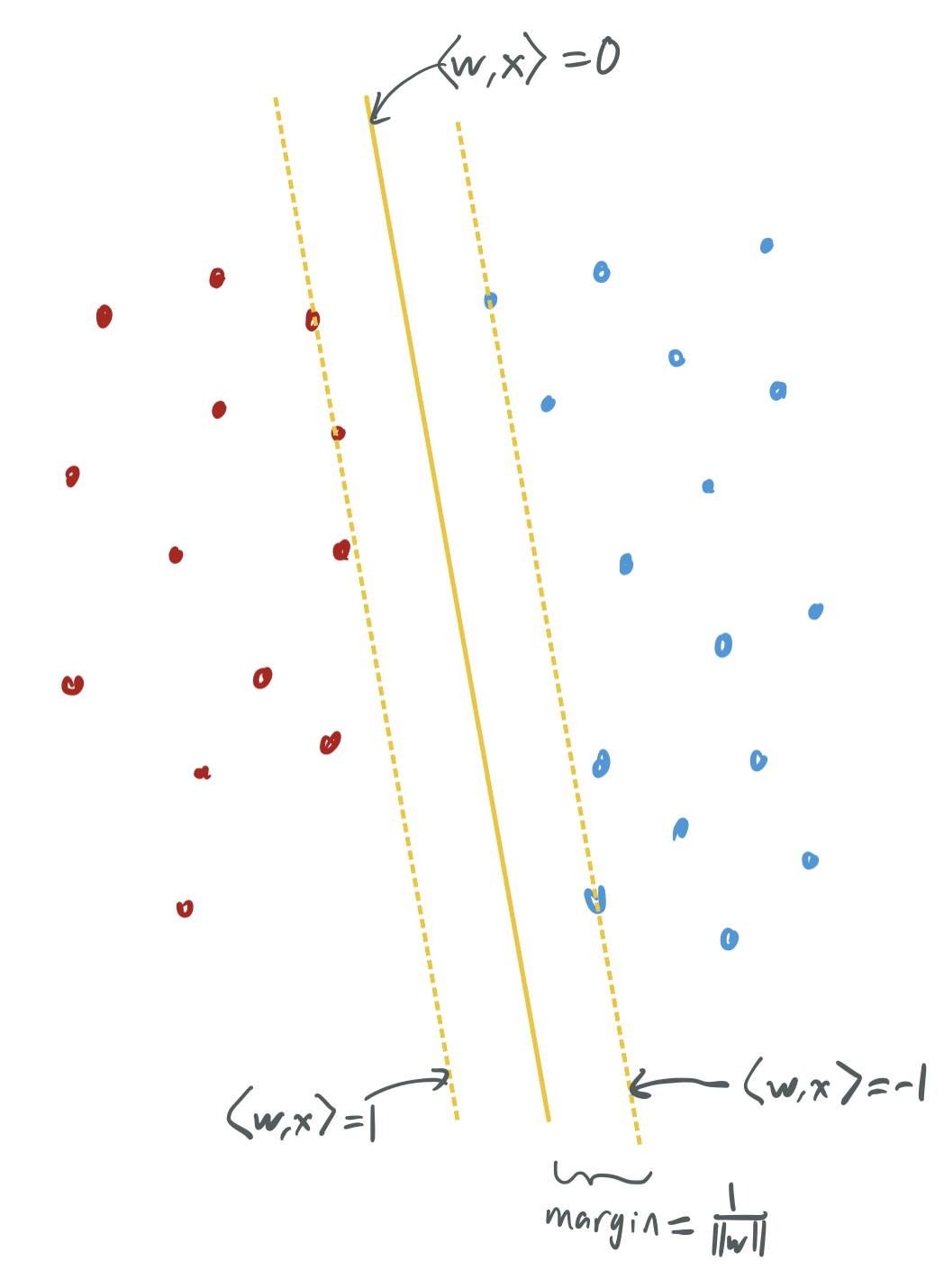
A key features of SVMs is that the classifier can also be defined by a subset of the training samples, the ones that lie exactly on the margin, i.e. have \(w_{SVM}^T x_i = y_i\). These are called the support vectors. If \(x_1, \dots, x_k\) are the support vectors of \(w_{SVM}\), then \(w_{SVM} = \sum_{i=1}^k \alpha_i x_i\) for some \(\alpha \in \mathbb{R}^k\). Traditionally, bounds on the generalization powers of SVMs depend on the number of support vectors: fewer support vectors means an intrinsically “simpler” model, which indicates a higher likelihood that the model is robust and generalizes well to new data.
Support vector proliferation, or OLS = SVM
By looking back at the two optimization problems for high-dimensional OLS and SVMs, the two are actually extremely similar. In the case where the OLS problem has binary labels \(\{-1, 1\}\), the two are exactly the same, except that the SVM problem has inequality constraints and OLS has equality. Therefore, in the event that the optimal SVM solution \(w_{SVM}\) satisfies each inequality constraint with equality, then \(w_{SVM} = w_{OLS}\). Because a constraint is satisfied with equality if and only if the corresponding sample is a support vector, \(w_{SVM} = w_{OLS}\) if and only if every training sample is a support vector. We call this phenomenon support vector proliferation (SVP) and explore it as the primary goal of our paper. Our contributions involve studying when SVP occurs and when it does not, which has implications for SVM generalization and the high-dimensional behavior of both models.
Why care about SVP and what is known?
The study of support vector proliferation has previously provided bounds on generalization behavior of high-dimensional (or over-parameterized) SVMs, and our tighter understanding of the phenomenon will make future bounds easier. In particular, the paper MNSBHS20 (which includes Daniel as an author) bounds the generalization of high-dimensional SVMs by (1) using SVP to relate SVMs to OLS and (2) showing that OLS with binary outputs has favorable generalization guarantees under certain distributional assumptions, similar to those of BLLT19. Specifically, they show that SVP occurs roughly when \(d = \Omega(n^{3/2} \log n)\) for the case where the variances of each feature are roughly the same.
This paper does not answer how tight the phenomenon is, leaving open the question of when (as a function of \(d\) and \(n\)) will SVP occur and when will it not. This question was partially addressed in a follow-up paper, HMX21 by Daniel, Vidya Muthukumar, and Mark Xu. The show roughly that SVP occurs (for a broad family of data distributions) when \(d = \Omega(n \log n)\) and that it does not occur (for a narrow family of distributions) when \(d = O(n)\), leaving open a logarithmic gap. Our paper closes this gap and considers a broader family of data distributions.
SVM generalization has also been targeted by CL20 and others using approaches that rely not on SVP by on the relationship between SVMs and gradient descent. Specifically, they rely on a fact from SHNGS18, which shows that gradient descent applied to logistic losses converges to a maximum-margin classifier. This heightens the relevance of support vector machines, since more sophisticated models may trend towards the solutions of hard-margin SVMs when trained with gradient methods. Thus, our exploration of SVP and how it relates minimum-norm and maximum-margin models may have insights about the high-dimensional behavior of other learning algorithms that rely on implicit regularization.
What do we prove?
Before jumping into our results, we introduce our data model and explain what HMX21 already explained in that setting.
Data model
We consider two settings each of which have independent random features for each \(x_i\) and fixed labels \(y_i\).
Isotropic Gaussian sample: For fixed \(y_1, \dots, y_n \in \{-1, 1\}\), each sample \(x_1, \dots, x_n \in \mathbb{R}^d\) is drawn independently from a multivariate spherical (or isotropic or standard) Gaussian \(\mathcal{N}(0, I_d)\).
Anisotropic subgaussian sample: For fixed \(y_1, \dots, y_n \in \{-1, 1\}\), each sample \(x_i\) is defined to be \(x_i = \Sigma^{1/2} z_i\), where each \(z_i\) is drawn independently from a 1-subgaussian distribution with mean zero and \(\Sigma\) is a diagonal covariance matrix with entries \(\lambda_1 > \dots > \lambda_d\). Hence, \(\mathbb{E}[x_i] = 0\) and \(\mathbb{E}[x_i x_i^T] = \Sigma\).
If the latter model has a Gaussian distribution, then \(\Sigma\) can be permitted to be any positive definite covariance matrix with eigenvalues \(\lambda_1, \dots, \lambda_n\) due to the rotational symmetry of the Gaussian.
We consider the regime \(d \gg n\) in order to ensure that the data are linearly separable with extremely high probability, which is acceptable because the paper is focused on the study of the over-parameterized regime.
The anisotropic data model requires using dimension proxies rather than \(d\) on occasion, because the rapidly decreasing variances could cause the data to have a much smaller effective dimension. (Similar notions are explored in HMX21 and over-parameterization papers like BLLT19.) We use two notions of effective dimension: \(d_\infty = \frac{\|\lambda\|_1}{\|\lambda\|_\infty}\) and \(d_2 = \frac{\|\lambda\|_1^2}{\|\lambda\|_2^2}\). Note that \(d_\infty \leq d_2 \leq d\).
Contributions of HMX21
HMX21 proves two bounds: an upper bound on the SVP threshold for an anisotropic subgaussian sample and a lower bound on the SVP threshold for an isotropic gaussian sample.
Theorem 1 [HMX21]: For an anisotropic subgaussian sample, if \(d_\infty = \Omega(n \log n)\), then SVP occurs with probability at least \(0.9\).
Theorem 2 [HMX21]: For an isotropic Gaussian sample, if \(d = O(n)\), then SVP occurs with probability at most \(0.1\).
This leaves open two obvious technical questions, which we resolve: closure of the \(n\) vs \(n \log n\) gap and generalization of Theorem 2 to handle the anisotropic subgaussian data model. We give these results, and a few others about more precise thresholds, in the next few sections.
Result #1: Closing the gap for the isotropic Gaussian case
We close the gap between the two HMX21 bounds by showing that the critical SVP threshold occurs at \(\Theta(n \log n)\). The following is a simplified version of our Theorem 3, which is presented in full generality in the next section.
Theorem 3 [Simplified]: For an isotropic Gaussian sample, if \(d = O(n \log n)\) and \(n\) is sufficiently large, then SVP occurs with probability at most \(0.1\).
In the version given in the paper, there is also a \(\delta\) variable to represent the probability of SVP occuring; for simplicity, we leave this out of the bound in the blog post.
We’ll discuss key components of the proof of this theorem later on in the blog post.
Result #2: Extending the lower bound to the anisotropic subgaussian case
Our version of Theorem 3 further extends Theorem 2 to the anisotropic subgaussian data model, at the cost of some more complexity.
Theorem 3 : For an anisotropic subgaussian sample, if \(d_2 = O(n \log n)\), \({d_\infty^2}/{d_2} = {\|\lambda\|_2^2}/{\|\lambda\|_\infty^2} = \Omega(n)\), and \(n\) is sufficiently large, then SVP occurs with probability at most \(0.1\).
The second condition ensures that the effective number of points with high variance is at least as large as \(n\). If it were not, then a very small number of features would have an outsize influence on the outcome of the problem, making it effectively a low-dimensional problem where the data are unlikely even to be linearly separable.
The first condition is slightly loose in the event that \(d_2 \gg d_\infty\), since Theorem 1 depends on \(d_\infty\) rather than \(d_2\).
Result #3: Proving a sharp threshold for the isotropic Gaussian case
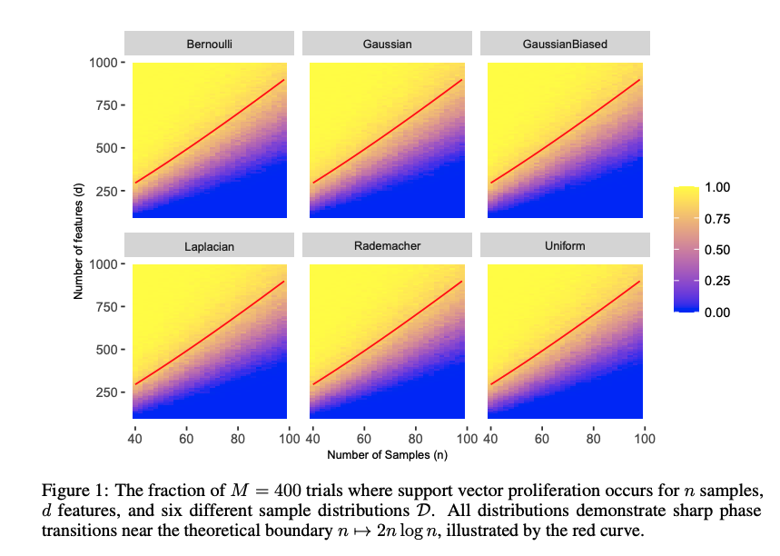
Returning to the simple isotropic Gaussian regime, we show a clear threshold in the regime where \(n\) and \(d\) become arbitrarily large. Theorem 4 shows that the phase transition occurs precisely when \(d = 2n \log n\) in the asymptotic case. Check out the paper for a rigorous asymptotic statement and a proof that depends on the maximum of weakly dependent Gaussian variables.
Note: One nice thing about working with a statistician is that we have different flavors of bounds that we like to prove. As a computer scientist, I’m accustomed to proving Big-\(O\) and Big-\(\Omega\) bounds for finite \(n\) and \(d\) in Theorem 3, while hiding foul constants behind the asymptotic notation. On the other hand, Navid is more interested in the kinds of sharp trade-offs that occur in infinite limits, like those in Theorem 4. Our collaboration meant we featured both!
Result #4: Suggesting the threshold extends beyond that case
While we only prove the location of the precise threshold and the convergence to that threshold for the isotropic Gaussian regime, we believe that it persists for a broad class of data distributions, including some that are not subgaussian. Our Figure 1 visualizes this universality by visualizing the fraction of trials on synthetic data where support vector proliferation occurs when the samples are drawn from each type of distribution.
Conjecture: Generalization to \(L_1\) (and \(L_p\)) models
We conclude by generalizing the SVM vs OLS problem to different norms and making a conjecture that the SVP threshold occurs when \(d\) is much larger for the \(L_1\) case. For the sake of time, that’s all I’ll say about it here, but check out the paper to see our formulation of the question and some supporting empirical results.
Proof of Result #1
I’ll conclude the post by briefly summarizing the foundations of our proof of the simplified version of Theorem 3. This was an adaptation of the techniques employed by HMX21 to prove Theorem 2, but it required a more careful approach to handle the lack of independence among a collection of random variables.
Equivalence lemma
Both papers rely on the same “leave-one-out” equivalence lemma for their upper and lower bounds. We prove a more general version in our paper based on geometric intuition, but I give only the simpler one here.
Let \(y_{\setminus i} = (y_1, \dots, y_{i-1}, y_{i+1}, \dots, y_n) \in \mathbb{R}^{n-1}\) and \(X_{\setminus i} = (x_1, \dots, x_{i-1}, x_{i+1}, \dots, x_n) \in \mathbb{R}^{(n-1) \times d}\).
Lemma 1: Every training sample is a support vector (i.e. SVP occurs and OLS=SVM) if and only if \(u_i := y_i y_{\setminus i}^T (X_{\setminus i} X_{\setminus i}^T)^{-1} X_{\setminus i} x_i < 1\) for all \(i \in [n]\).
This lemma looks a bit ugly as is, so let’s break it down and explain hazily why the connection these \(u_i\) quantities connect to whether a sample is a support vector.
- Noting that \(X_{\setminus i}^\dagger = (X_{\setminus i} X_{\setminus i}^T)^{-1} X_{\setminus i}\) when \(d \gg n\) and referring back to the optimization problems from before, we can let \(y_{\setminus i}^T (X_{\setminus i} X_{\setminus i}^T)^{-1} X_{\setminus i} := w_{OLS, i}^T\), because it represents the parameter vector obtained by running OLS on all of the training data except \((x_i, y_i)\).
- Then, \(u_i = y_i x_i^T w_{OLS, i}\), which is the margin of the “leave-one-out” regression on the left out sample.
- If \(u_i \geq 1\), then the OLS classifier on the other \(n-1\) samples already classifies \(x_i\) correctly by at least a unit margin. If the \(w_{OLS, i} = w_{SVM, i}\), then it suffices to take \(w_{SVM} = w_{OLS, i}\) without adding a new support vector for \(x_i\) and without increasing the cost of the objecting. Hence, the condition means that the partial solution offers proof that not everything needs to be a support vector.
- If \(u_i < 1\), then \(x_i\) is not classified to a unit margin by \(w_{OLS, i}\). Therefore, adding \((x_i, y_i)\) back into the training set requires modifying the parameter vector; since the vector would then depend on \(x_i\), making \(x_i\) a support vector of \(w_{SVM}\).
The remainder of the proof involves considering \(\max_i u_i\) and asking how large it must be.
Assuming independence
In the Gaussian setting where \(X_{\setminus i}\) is fixed, \(u_i\) is a univariate Gaussian random variable of mean 0 and variance \(y_{\setminus i}^T (X_{\setminus i} X_{\setminus i}^T)^{-1} X_{\setminus i} X_{\setminus i}^T (X_{\setminus i} X_{\setminus i}^T)^{-1}y_{\setminus i} = y_{\setminus i}^T (X_{\setminus i} X_{\setminus i}^T)^{-1} y_{\setminus i}\).
Because \(\mathbb{E}[x_j^T x_j] = d\), it follows that \(\mathbb{E}[X_{\setminus i} X_{\setminus i}^T] = d I_{n-1}\) and that the eigenvalues of \(X_{\setminus i} X_{\setminus i}^T\) are concentrated around \(d\) with high probability. As a result, the eigenvalues of \((X_{\setminus i} X_{\setminus i}^T)^{-1}\) are concentrated around \(1/d\), and the variance of \(u_i\) is roughly \(\frac{1}{d} \|y_{\setminus i}\|_2 = \frac{n-1}d\).
If we assume for the sake of simplicity that \(u_i\) are all independent of one another, then the problem becomes easy to characterize. It’s well-known the maximum of \(n\) Gaussians of variance \(\sigma^2\) concentrates around \(\sigma \sqrt{2 \log n}\). Hence, \(u_i\) will be roughly \(\sqrt{2(n-1)\log(n) / d}\) with high probability. If \(d = \Omega(n \log n)\), then \(\max_{u_i} < 1\) with high probability and SVP occurs; if \(d = O(n \log n)\), then SVP occurs with with vanishingly small probability.
Overcoming dependence
The key problem with the above paragraphs is that the random variables \(u_1, \dots, u_n\) are not independent of one another. They all depend on all of the data \(x_1, \dots, x_n\), and the core technical challenge of this result is to tease apart this dependence. To do so, we rely on the fact that \(X_{\setminus i} X_{\setminus i}^T \approx d I_{n-1}\) and define a subsample of \(m \ll n\) points to force an independence relationship. Specifically, we rely on the decomposition \(u_i = u^{(1)}_i + u^{(2)}_i + u^{(3)}_i\) for \(i \in [m]\) where:
- \(u^{(1)}_i = y_i y_{\setminus i}^T((X_{\setminus i} X_{\setminus i}^T)^{-1} - \frac1d I_{n-1}) X_{\setminus i} x_i\) represents the gap between the gram matrix \(X_{\setminus i} X_{\setminus i}^T\) and the identity.
- \(u^{(2)}_i = \frac1d y_i y_{[m] \setminus i} X_{[m] \setminus i} x_i\) is the component of the remaining term (\(\frac1d y_i y_{\setminus i} X_{\setminus i} x_i\)) that depends exclusively on the subsample \([m]\).
- \(u^{(3)}_i = \frac1d y_i y_{\setminus [m]} X_{\setminus [m]} x_i\) is the component that depends only on \(x_i\) and on samples outside the subsample. Critically, \(u^{(3)}_1, \dots, u^{(3)}_m\) are independent, conditioned on the data outside the sample, \(X_{\setminus [m]}\).
To show that SVP occurs with very small probability, we must show that \(\max_i u_i \geq 1\) with high probability. To do so, it’s sufficient to show that (1) for all \(i\), \(|u^{(1)}_i| \leq 1\); (2) for all \(i\), \(|u^{(2)}_i| \leq 1\); and (3) \(\max_i u^{(3)}_i \geq 3\). The main technical lemmas of the paper apply Gaussian concentration inequalities to prove (1) and (2), and leverage the independence of the \(u^{(3)}_i\)’s to prove that their maximum is sufficiently large.
This requires somewhat more advanced techniques, such as the Berry-Esseen theorem, for the subgaussian case.
What’s next?
We think the significance of this result is the tying together of seemingly dissimilar ML models by their behavior in over-parameterized settings. We think some immediate follow-ups on this include investigations into the generalized \(L_p\) SVM and OLS models, but further work could also work along the lines of SHNGS18, by connecting “classical” ML models (like maximum-margin models) to the implicit regularization behavior of more complex models.
Thanks for reading this post! If you have any questions or thoughts (or ideas about what I should write about), please share them with me.
Comments