Whoops, six months just went by without a blog post. The first half of 2022 has been busy, and I hope to catch up on writing about some of the other theory papers I’ve worked on, the climate modeling project I’m currently involved in at the Allen Institute for AI, random outdoor adventures and hikes in Seattle, and some general reflections on finishing my third year and having a “mid-PhD crisis.” For now though, here’s a summary of a paper that appeared at COLT (Conference on Learning Theory) a couple weeks ago in London. This is similar to my two previous summary posts, which are meant to break down papers I’ve helped write into more easily-digestible chunks. As always, questions and feedback are greatly appreciated.

Last August, I attended COLT 2021 for the first time to present my first paper as a graduate student, which I wrote along with my advisors, Rocco Servedio and Daniel Hsu, and my fellow PhD student, Manolis Vlatakis-Gkaragkounis. COLT was one of the first conferences to be in-person, so I was fortunate enough to spend a week in Boulder, CO and get to know other ML theory researchers over numerous talks and gorgeous hikes. This year, the same set of authors sent a second paper to COLT 2022—in part due to our desire for funded travel to London—and I was there last week to present it in-person.

My talk was a little silly. Since I presented it on July 4th, I had this whole American Revolution analogy, about the four of us thwarting the attempts of British soldiers to spy on the continental army. I’ll make a few references to that in this post.

While both this paper and my COLT 2021 paper are machine learning theory papers, they differ substantially in their areas of focus: The paper last year (which I’ll call HSSV21) was about the approximation capabilities and limitations of shallow neural networks This year’s paper (HSSV22) is completely detached from neural networks and instead focuses on a “classical learning theory” question about resource-intensive an algorithm must be to learn a seemingly-simple family of functions. Indeed, this is different from all of the other papers I’ve worked on in grad school, as they all focus on neural networks and relevant learning theory in various ways: approximation, over-parameterization, approximation again, and implicit biases.

What does this paper actually do?

The easiest way to explain what the paper does is by breaking down its title–Near-Optimal Statistical Query Lower Bounds for Agnostically Learning Intersections of Halfspaces with Gaussian Marginals–piece by piece and discussing what each piece means.

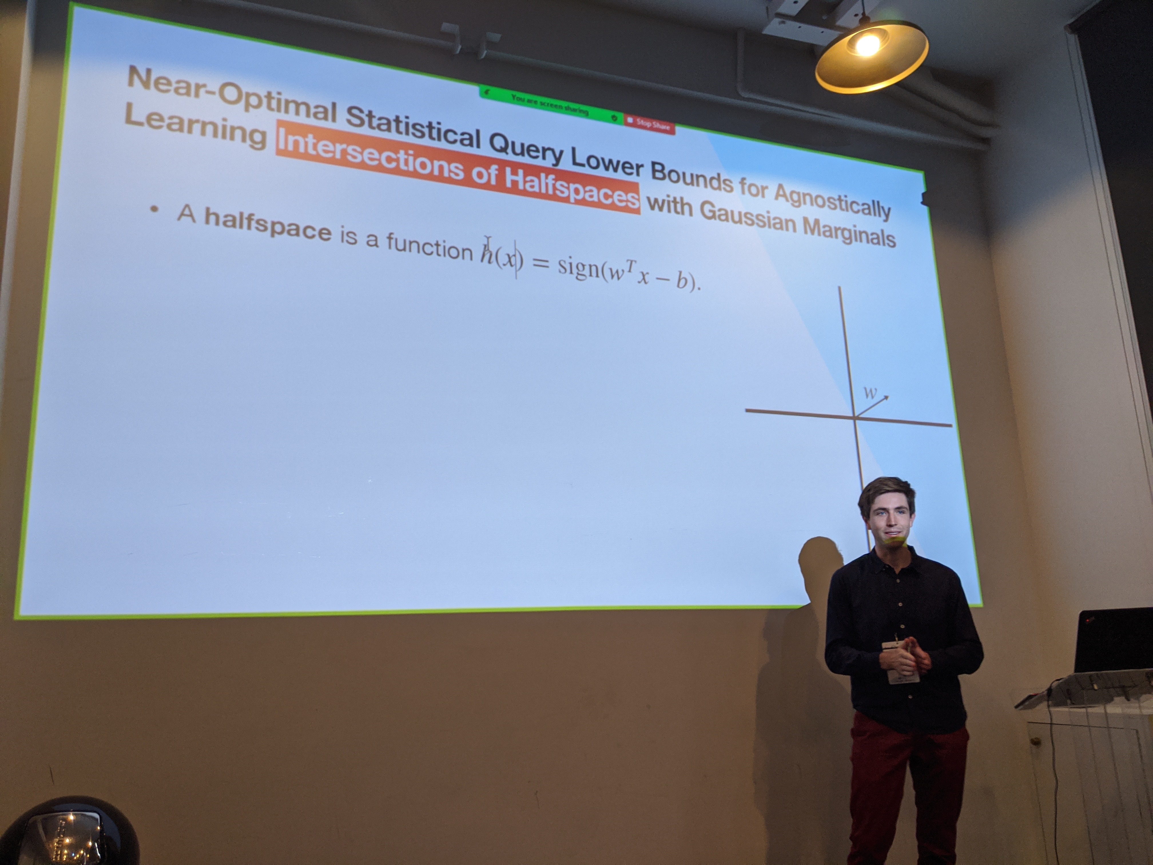
Near-Optimal Statistical Query Lower Bounds for Agnostically Learning Intersections of Halfspaces with Gaussian Marginals

To formalize a classification learning problem, we draw labeled samples \((x, y)\) with input \(x \in \mathbb{R}^n\) and label \(y \in \{\pm 1\}\) from some distribution \(\mathcal{D}\). We are given a training set of \(m\) independent samples \((x_1, y_1), \dots, (x_m, y_m)\) from that distribution, and our goal is to infer some hypothesis function \(f: \mathbb{R}^n \to \{\pm1\}\) that not only correctly categorizes most (if not all) of the training sample but also generalizes to new data by having a loss \(L(f) = \mathbb{E}_{(x, y) \sim \mathcal{D}}[{1}\{f(x) \neq y\}]\) that is close to zero.

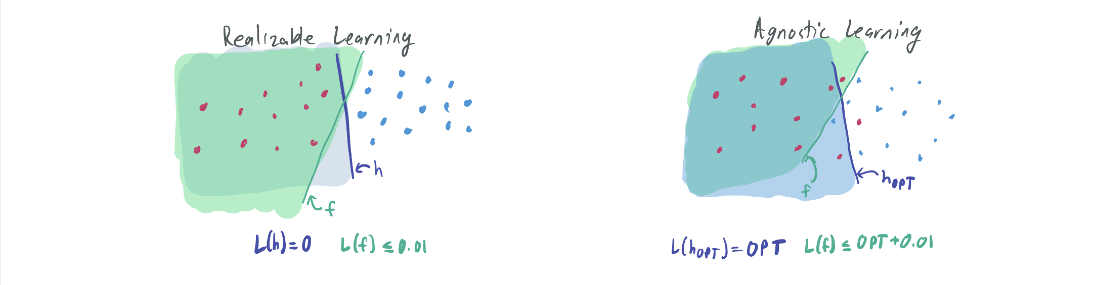
Realizable learning refers to a category of classification problems in which there is guaranteed to exist a hypothesis in some set \(\mathcal{H}\) that perfectly classifies all data. That is, there exists \(h \in \mathcal{H}\) such that \(y = h(x)\) always. We consider a realizable learning algorithm successful if the loss of its returned predictor \(f\) is not much larger than zero, that is \(L(f) \leq \epsilon\) for some small \(\epsilon > 0\).

Note that \(f\) is not necessarily contained in \(\mathcal{H}\). If we require \(f\) to be in \(\mathcal{H}\), then the problem is known as proper, but that is a separate type of learning problem that we don’t consider in the paper or this blog post.

Agnostic learning is a more difficult regime where there may not exist such an \(h\) that perfectly classifies every sample. As a result, the best we can do is to obtain a loss that is not much larger than the optimal loss among all classifiers in \(\mathcal{H}\), which may be much larger than 0. That is, \(L(h) \leq \epsilon + \mathrm{OPT}\) where \(\mathrm{OPT} = \min_{h \in \mathcal{H}} L(h)\).

For simplicity in this blog post, we’re going to let \(\epsilon = 0.01\) throughout. We can prove everything we need for general \(\epsilon\); check out the paper if you’re interested in that.

In this paper, we focus exclusively on the agnostic setting. Agnostic learning is a “harder” problem in that it strictly generalizes the realizable class, and some hypothesis classes (such as parities) have efficient algorithms for the realizable case but none known for the agnostic case.

at least as many samples and time are needed to agnostically learn a hypothesis family \(\mathcal{H}\) as is needed to realizably learn it.

For our themed talk, we recast the problem of learning as the challenge of spying on an army to determine where troops are concealed. In this case, the spy receives information about specific locations at random (e.g. “there is a soldier at this location; there is not a soldier at that location”) and must infer a good estimate about where the rest of the army is likely to be based on these samples.

Near-Optimal Statistical Query Lower Bounds for Agnostically Learning Intersections of Halfspaces with Gaussian Marginals

A halfspace is a function that is positive on one side of a separating hyperplane and negative on the other. That is, \(h(x) = \mathrm{sign}(w^T x - b)\) for direction \(w \in \mathbb{R}^n\) and bias \(b \in \mathbb{R}\). The family of all halfspaces \(\mathcal{H}_1 = \{x \mapsto \mathrm{sign}(w^T x - b) : w, b\}\) is well-established in ML theory via linear separability.

By combining the definition of a halfspace with those of the two learning regimes discussed above, we can see clearly how they differ. Because the realizable setting requires the existence of some \(h \in \mathcal{H}_1\) that perfectly classifies the data, the problem of realizably learning halfspaces always involves having linearly separable data. An algorithm realizably learns halfspaces if it returns a function (not necessarily a halfspace!) with loss at most 0.01. This can be done with a maximum margin support vector machine (SVM) with \(\mathrm{poly}(n)\) sample and time complexity.

On the other hand, agnostically learning intersections of halfspaces introduces no dataset restrictions and asks the learner to pick a hypothesis with loss no more than 0.01 plus that of the best possible halfspace.

Near-Optimal Statistical Query Lower Bounds for Agnostically Learning Intersections of Halfspaces with Gaussian Marginals

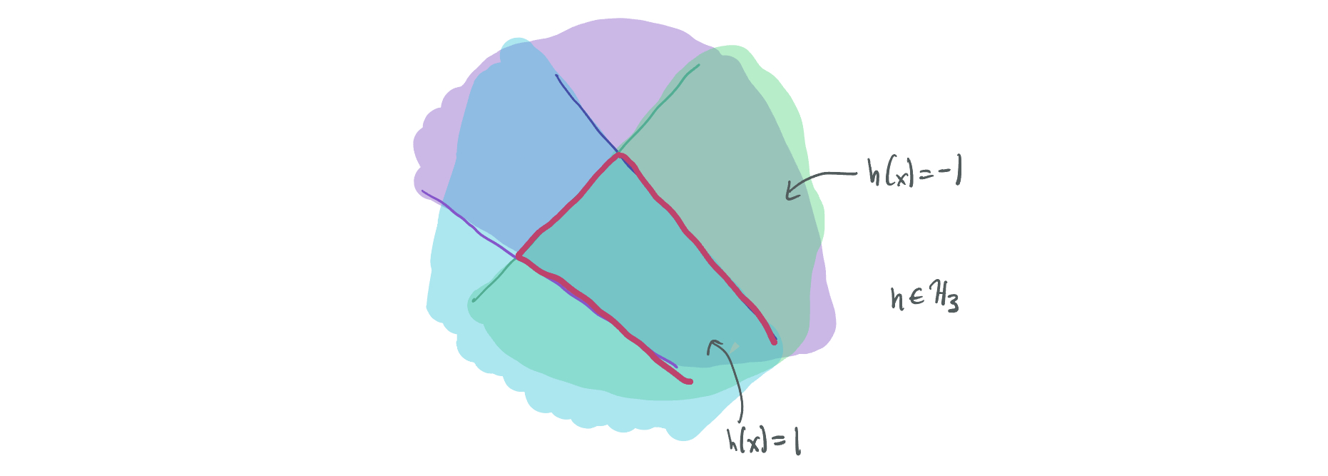
Likewise, an intersection of halfspaces is a function that evaluates to 1 if and only if \(k\) different halfspaces all are 1, i.e. \(h(x) = \min_{i \in [k]} \mathrm{sign}(w_i^T x - b_i)\) and \(\mathcal{H}_k = \{x \mapsto \min_{i \in [k]} \mathrm{sign}(w_i^T x - b_i): w_1, \dots, w_k, b_1, \dots, b_k\}\).

As will be discussed soon, the problem of learning intersections of halfspaces is also well-studied, in part due to the idea of the credit allocation problem. The idea of this problem is that a common classification regime might be one where a positive classification is only obtained if a larger number of Boolean conditions are satisfied. For instance, risk assessment decisions may depend more on ruling out individuals who display any of a number of risk factors without notifying them of which condition they failed to meet. If each of those decision rules is a simple (in this case, a halfspace) combination of one’s information, then the task of learning intersections of halfspaces is relevant to learning in this very specific case.

In addition, for our extremely applicable American Revolution application, the continental army is primarily capable of arranging its troops in \(\mathbb{R}^n\) space behind a collection of battle lines, a.k.a. within an intersection of halfspaces. As such, it’s the goal of the British spies to learn the troop formations by trying to have an estimate that is nearly as good as the intersection of halfspaces that most accurately categorizes where soldiers are and where they are not.

Near-Optimal Statistical Query Lower Bounds for Agnostically Learning Intersections of Halfspaces with Gaussian Marginals

In the definition of agnostic and realizable learning, we did not restrict the data distribution \(\mathcal{D}\). Now, we’re going to further simplify things by considering only one of the easiest cases, where the probability distribution is the \(n\)-dimensional multivariate standard Gaussian, \(\mathcal{N}(0, I_n)\).

Why do we focus on this simple case? Two quick things:

Recall that if we’re proving lower bounds (or showing that solving a problem is highly resource-intensive) than it’s more difficult to prove a result for an “easier” distribution. This means that there doesn’t even exist an algorithm for this very natural data distribution, which is more interesting than showing the same for some very obscure distribution.
The problem of agnostically learning halfspaces is already known to be very difficult to solve in the case when distributional assumptions are not made. See this paper by Sherstov, which shows that even learning \(\mathcal{H}_2\) requires \(\exp(n)\) time (under cryptographic assumptions).

Near-Optimal Statistical Query Lower Bounds for Agnostically Learning Intersections of Halfspaces with Gaussian Marginals

I’m going to tweak the learning model once again, this time replacing the reliance on explicit samples drawn from a probability distribution with the statistical query (SQ) model where the learning algorithm instead requests information about the learning problem in the form of queries and receives information with some accuracy guarantee.

That is, an SQ learning algorithm is one that makes \(M\) queries of the form \((q, \tau)\) where \(q: \mathbb{R}^n \times \{\pm1\} \to [-1, 1]\) is a bounded query function and \(\tau > 0\) is the allowable error or tolerance. We say that an SQ algorithm is efficient if its query count \(M\) and inverse tolerance \(1 / \tau\) are polynomial in \(n\).

Our British intelligence system then—rather than obtaining individual data points about whether a soldier is a present at a given location—asks its comprehensive network of spies a question about some aggregate property of the entire army and receives an accurate response.

To be clear, no one actually operates within the statistical query model, where we ask questions and obtain (potentially adversarial) answers; the whole point of ML is that predictions are purely based on data. But it’s a useful model for understanding ML algorithms and their limitations.

Why do we use the SQ model? We analyze it because it’s similar in functionality to the standard sample-based model, and its limitations are much easier to understand mathematically.

Most sample-based learning algorithms are SQ learning algorithms. Many learning algorithms (such as stochastic gradient descent and ordinary least squares (OLS) regression) depend on using a sufficiently large number of samples to estimate certain expectations and moments. For instance, gradient descent involves using a batch of \(m'\) samples to estimate the expected gradient \(\mathbb{E}_{(x, y)}[\nabla_\theta \ell(y, h_\theta(x))]\) of the loss function \(\ell\) for a parameterized function \(h_\theta\) (typically a neural network) and using this to iteratively update the parameter \(\theta\). The gradient estimate is essentially the empirical average, \(\sum_{i=1}^{m'} \nabla_\theta \ell(y_i, h_\theta(x_i))\) (it may also include other regularization terms or a momentum term, but we’ll ignore that now).

We can implement a similar algorithm in the SQ model by replacing each gradient computation with the query \(q_j(x, y)= \nabla_{\theta_j} h_\theta(y, h_\theta(x))\) for each \(j \in [n]\) and a small tolerance \(\tau\). Because both algorithms provide similar estimates of the same quantity, we can use the SQ model to have the same effect as the sample-based model. There are a few notable exceptions of sample-based learning algorithms that cannot be implemented in the SQ model, such as the Gaussian elimination algorithm for learning parities; indeed no SQ algorithm can learn parities. However, Gaussian elimination does not work when the data are noisy (i.e. a small fraction of samples are labeled incorrectly), and cryptographic hardness results suggest that there is no such sample-based algorithm for learning parities.

Every SQ learning algorithm can be implemented in the sample-based model. How? Suppose we have an SQ learning algorithm with \(M\) queries of tolerance \(\tau\). We can simulate the \(i\)th query \(q_i\) with \(m_i = 2 \ln(100M ) / \tau^2\) samples \((x_1, y_1), \dots (x_{m_i}, y_{m_i})\) by outputting some \(\hat{Q}_i := \frac1{m_i} \sum_{i=1}^{m_i} q(x_i, y_i)\). By Hoeffding’s inequality, with probability at least \(1 - \frac{1}{100M}\),

\[|\mathbb{E}[q_i(x, y)] - Q_i| \leq \sqrt{2 \ln (100M) / m_i} = \tau.\]

As a result, the outcome \(Q_i\) of every query \(q_i\) is within the desired tolerance \(\tau\) with probability at least \(0.99\), which makes the sample-based algorithm work at simulating the SQ algorithm with \(m := M \cdot m_i = 2M \ln(M / 100) / \tau^2\) samples. If \(M\) and \(\frac{1}\tau\) are polynomial, then so is the total number of samples \(m\). The run-time of the algorithm is additionally polynomial.

Near-Optimal Statistical Query Lower Bounds for Agnostically Learning Intersections of Halfspaces with Gaussian Marginals

In our analogy, we’re more interested in helping the revolutionaries defeat the British by outwitting their master spy web. That is, we want to understand the limitations of their ability to query their spy network for information about where American troops are located. In doing so, the Americans can understand what kind of troop formations to consider in order to make it impossible for the Brits to detect their soldiers.

As mentioned before, an SQ algorithm is efficient if \(\max(M, 1/\tau) = \mathrm{poly}(n)\). Hence, we can show hardness results in the SQ model by showing that any algorithm that solves a problem (in our case, the problem of agnostically learning intersections of halfspaces under Gaussian marginals) requires that either \(M\) or \(1 / \tau\) grows super-polynomially in \(n\).

The SQ model is particularly useful for hardness results because it’s easier to prove limitations of time and sample complexity than in the sample-based model. Consider the above construction, where the sample-based model is used to implement an SQ algorithm. Because the algorithm simulates every query, if \(M\) is exponential, then the time complexity of the sample-based algorithm must also be exponential. Likewise, if \(1 / \tau\) is exponential, then the number of samples \(m_i\) needed for each query is exponential, which corresponds to exponential sample complexity. Thus, hardness results in the SQ model roughly imply that there won’t exist any other “reasonable” learning algorithm that solves the problem with polynomial time or samples.

This is nice because it’s typically very hard to prove lower bounds on runtime for learning algorithms in the sample-based model. It’s mathematically simpler to prove information-theoretic bounds on sample complexity for certain cases, but these only apply to very hard learning problems where no algorithm with a polynomial number of samples exists, let alone one with a polynomial runtime. However, there are conjectured problems with computational-statistical gaps, where the problem can be solved with a polynomial number of samples at a very large time complexity cost. Proving these time complexity limitations is considerably more difficult in the sample-based model; the main known approach is to use cryptographic hardness assumptions (like the unique shortest vector problem used for intersections of halfspaces in this Klivans and Sherstov paper), but these are complicated to employ and rely on assumptions that are likely but not certainly true.

SQ-based lower bounds provide a good way to suggest that a learning problem will not be able to be learned without a large runtime. Since the model is not a perfect correspondence to the sample-based model, SQ-hardness is not a guarantee that there will be no efficient algorithm, but it does promise that most nice and robust algorithms will be unable to solve the problem with an efficient runtime.

Near-Optimal Statistical Query Lower Bounds for Agnostically Learning Intersections of Halfspaces with Gaussian Marginals

Putting together all of the past snippets, we conclude that the theorem this paper proves will be of the following form:

Theorem: For sufficiently large \(n\) and \(k \leq ???\), any statistical query algorithm with \(M\) queries of tolerance \(\tau\) that agnostically learns \(\mathcal{H}_k\) over samples with marginal distribution \(\mathcal{N}(0, I_n)\) requires either \(M \geq ???\) or \(\tau < ???\).

But what should replace the \(???\)’s? To get some intuition, we ask what it means to be “nearly optimal.”

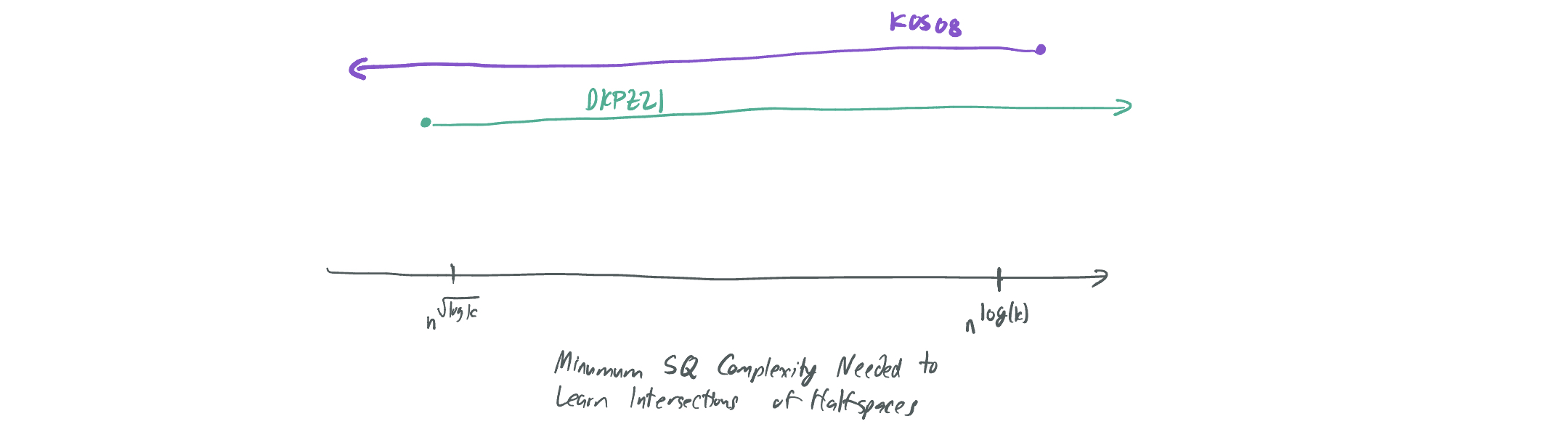
Let’s first start with a positive result, or an algorithm showing that something is possible for this problem. In 2008, Klivans, O’Donnell, and Servedio published a sample-based algorithm that agnostically learns \(k\) intersections of halfspaces in \(n\) dimensions with \(n^{O(\log k)}\) time and sample complexity. We’ll refer to this as “KOS08.” In the talk, I made the three of them former redcoats from the Seven Years War who developed British espionage techniques for use against their French enemies.

Critically, their algorithm can be implemented in the SQ model with \(M = n^{O(\log k)}\) and \(\tau = n^{-O(\log k)}\), which means the SQ lower bounds to be discussed limit improvement on this algorithm.

How does their approach work? The proceed in roughly three steps:

They show that any intersection of \(k\) halfspaces has a Gaussian surface area of at most \(O(\sqrt{\log k})\). (Because an intersection of \(k\)-halfspaces is a convex set, we can think of the function as an \(n\)-dimensional polytope with an \((n-1)\)-dimensional surface. The Gaussian surface area weights the surface according to the multivariate Gaussian probability distribution; surfaces closer to the origin then represent more “area” than surfaces further away.)
They show that any Boolean function \(f: \mathbb{R}^n \to \{\pm 1\}\) with Gaussian surface area at most \(s\) can be \(L_1\)-approximated by a polynomial \(p\) of degree \(O(s^2)\). (That is, \(\|f - p\|_2 = \mathbb{E}_{x \sim \mathcal{N}(0, 1)}[|f(x) - p(x)|] \leq 0.01\).)
The actual algorithm consists of performing \(L_1\) polynomial regression, which finds the \(d\)-degree polynomial that best fits the training data with \(n^{O(d^2)}\) samples and time.

Hence, an intersection of \(k\) halfspaces can be approximated by a polynomial of degree \(O(\log(k))\), so \(L_1\) polynomial regression with \(n^{O(\log k)}\) samples will find a target function that satisfies the agnostic learning problem.

In addition, there is a known lower bound that was presented at COLT 2021 by Diakonikolas, Kane, Pittas, and Zarifis (DKPZ21), which shows that any SQ algorithm learning this problem for \(k = O(n^{0.1})\) requires at either \(M \geq 2^{n^{0.1}}\) or \(\tau \leq n^{\tilde\Omega(\sqrt{\log k})}\). In the talk, these were French soldiers, who helped the Americans fight the British and put their understanding of British espionage to good use.

How did they do it? We’ll discuss this more later on, but here are the brief steps:

[Theorem 3.5] They show that some \(k\)-dimensional intersection of \(k\) halfspaces \(f:\mathbb{R}^k \to \{\pm1\}\) cannot be weakly approximated by any polynomial of degree \(O(\sqrt{\log k})\), which makes it approximately resilient.
[Theorem 1.4] They consider different projections of that function from \(n\)-dimensional space, \(F_W(x) = f(W x)\) for \(W \in \mathbb{R}^{k \times n}\) with orthonormal rows. Two randomly selected such matrices \(W_1\) and \(W_2\) will yield \(F_{W_1}\) and \(F_{W_2}\) that are nearly orthogonal (see my notes on orthogonality for an overview), i.e. \(\mathbb{E}_{x \sim \mathcal{N}(0, I_n)}[F_{W_1}(x) F_{W_2}(x)] \approx 0\). Then, there exists a collection of \(n\)-dimensional functions with a high SQ dimension (reference, pg 4). By standard results about SQ dimension, these functions are hard for any SQ algorithm to distinguish without either many queries or extremely accurate queries.

By comparing the DKPZ21 result with the KOS08 result, one can observe a substantial gap between the two with respect to \(k\): KOS08 asserts that it’s possible to learn intersections of \(k\)-halfspaces with tolerance \(n^{-O(\log k)}\), and DKPZ21 asserts that it’s possible as long as the tolerance is at most \(n^{-\tilde\Omega(\sqrt{\log k})}\). This leaves open the question: What is the correct tolerance? Can the algorithm of KOS08 be improved to yield a better one that doesn’t require queries to be quite so accurate (and the resulting sample-based algorithm to require fewer samples)? Or is there a stronger lower bound than DKPZ21’s that indicates that the KOS08 algorithm is indeed optimal?

So what do we actually do?

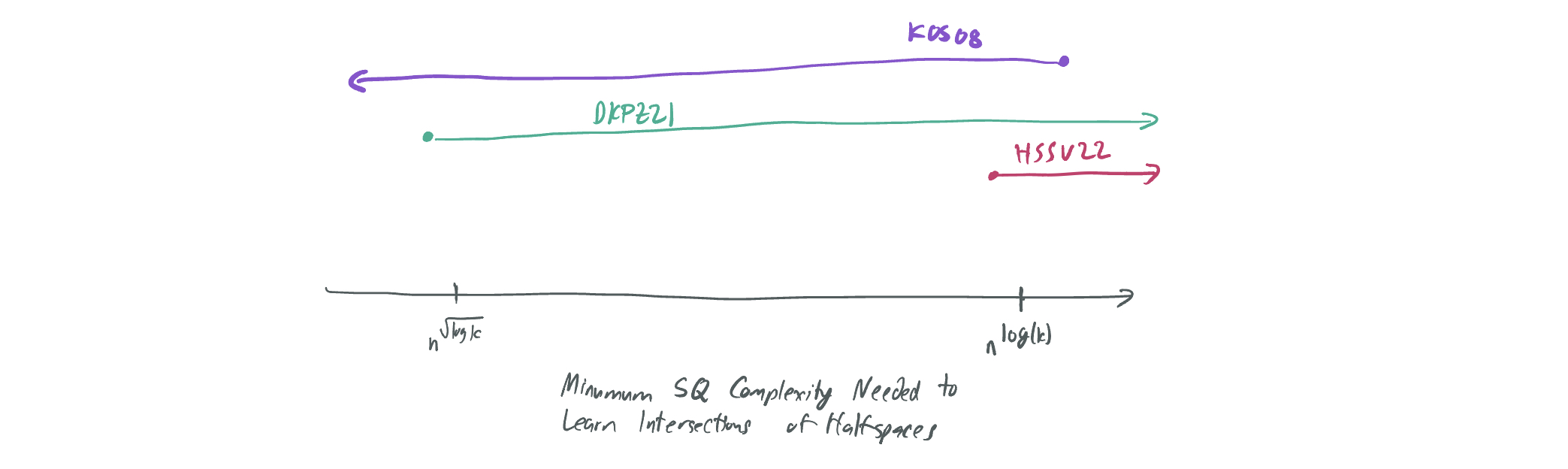
As one expects by looking at the title of our paper, we give a stronger lower bound and prove the near-optimality of the KOS08 algorithm.

Theorem: For sufficiently large \(n\) and \(k \leq 2^{O(n^{0.24})}\), any statistical query algorithm with \(M\) queries of tolerance \(\tau\) that agnostically learns \(\mathcal{H}_k\) over samples with marginal distribution \(\mathcal{N}(0, I_n)\) requires either \(M \geq 2^{\Omega(n^{0.1})}\) or \(\tau \leq n^{-\tilde\Omega(\log k)}\).

This result is almost identical to that of DKPZ21, save for the different dependence on \(\tau\). As a result, the tolerance of the KOS08 algorithm is optimal up to \(\log\log k\) factors in the exponent.

A few notes and caveats:

The similarity to the theorem of DKPZ21 is no coincidence; we use nearly the same method as they do, except we have a stronger bound on the approximate resilience of some intersection of \(O(k)\) halfspaces.
Our results are actually the combination of two theorems: one which gives an explicit construction of the “hard” intersection of halfspaces to learn but requires \(k \leq O(n^{0.49})\) and the other with a randomized construction. We’ll focus primarily on the former for the rest of this blog post… but you should read the paper to learn about how we adapted a construction from a COLT 2021 paper by De and Servedio for the second!
We don’t include the dependence of the target accuracy \(\epsilon\) in the above theorem, but it can be added by using a slight modification to the family of intersections of halfspaces that we consider. This involves a result by a Ganzburg paper from 2002 that establishes the \(L^1\) polynomial approximation properties of a single halfspace.

Okay, but who actually cares about this?

So yeah, this is a pretty abstract and theoretical result that is very far from neural networks or modern ML practice. But there are a few nice things about it that ideally should make this interesting to theoreticians, practitioners, and historians alike. (Okay, mostly just theoreticians.)

As mentioned before, there’s a connection to this credit allocation problem, where a large number of simple factors may individually be responsible for informing us about the outcome of the prediction. For instance, one might be denied a loan for failing one of many risk factors without being notified of the correct reason why. If one wanted to learn the model purely from labels—a collection of acceptances and rejections without rationales—this paper suggests that the problem is very hard if there may be a large number of aggregated factors, even if the factors are linear thresholds and the data follows a simple Gaussian distribution.
In general, proofs of optimality are nice because they tell us (1) that it’s not worth it investing further intellectual resources in trying to improve a solution and (2) there aren’t “hard instances” for an algorithm to handle that aren’t being handled well by the current algorithm.
Our proof techniques (which you’ll see shortly) seem to be an approach that isn’t widely used in this space, which uses functional analysis techniques to gradually transform one function into a similar one that has certain desirable properties.

How do we prove the result?

To discuss how our proof works, we compare the analysis of DKPZ21 to that of a paper that does something similar by Dachman-Soled, Feldman, Tang, Wan, and Wimmer from 2014 (DFTWW14). In the talk, these folks were expert Prussian soldiers, like Baron von Steuben, who trained the fledgling American army and passed along modern techniques in war/boolean function analysis.

Like DKPZ21 and HSSV22 (our paper) they prove a lower bound against agnostically learning a family of functions in the SQ model. Unlike us, they learn functions over the boolean cube, of the form \(\{\pm 1\}^n \to \{\pm1\}\). And instead of showing that the family of rotations of a single function \(f\) are hard to learn (\(\mathcal{H} = \{f(W x): W \in \mathbb{R}^{k \times d}\}\)) they consider juntas of \(f\), or functions that act on only a subset of the variables (\(\mathcal{H} = \{f(x_S): S \subset [n], |S| = k\}\), where \(x_S = (x_{s_1}, x_{s_2}, \dots, x_{s_k})\) for \(S = \{s_1, s_2, \dots, s_k\}\)).

Note: Our work fits into a cottage industry of results that translate results that apply to monotone functions on the boolean cube to convex sets in Gaussian space. There’s a pretty sophisticated analogy between the two that is summarized well in the intro of this “Convex Influencers” paper by Rocco, Anindya, and Shivam Nadmipalli (bagel_simp).

Their result proceeds in analogous steps to that of DKPZ21:

[Theorem 1.6] They show that a particular \(k\)-dimensional boolean function \(f: \{\pm1\}^k \to \{\pm1\}\)—in this case, a read-once DNF called \(\mathsf{Tribes}\), an OR-of-ANDs with no repeated variables in clauses, like \(f(x) = (x_1 \wedge x_2) \vee (x_3 \wedge \neg x_5) \vee x_7\)—cannot be approximated accurately by any polynomial of degree \(\tilde{O}(\log k)\), or that \(f\) is approximately \(\tilde{O}(\log k)\)-resilient.
[Theorem 2.3] They consider the family of juntas of that function \(\mathcal{H} = \{f(x_S): S \subset [n], \lvert S\rvert = k\}\) and show that this family contains a larger number of nearly orthonormal functions. This means the class has a high SQ dimension and is hence hard to learn without SQ queries of tolerance \(n^{-\tilde\Omega(\log k)}\).

If we contrast these steps with those of DKPZ21, a few things stand out:

The approximate resilience statement in (1) of DFTWW14 indicates that Tribes is inapproximable with higher-degree polynomials than (1) of DKPZ21 suggests that the intersection of halfspaces is. One way to improve DKPZ21 is to prove that their function is even harder to approximate with polynomials than they proved.
(2) of DKPZ21 is a more involved proof due to the continuity of the Gaussian setting, which involves some tricky maneuvers like the use of an infinite linear program.

Our result works by picking and choosing the best of each: we draw inspiration from the methods of DFTWW14 to improve the resilience bound of DKPZ21 to \(\Omega(\log k)\), while using (2) of DKPZ21 right out of the box. For the rest of this proof description, I’ll outline the basics of how we did that by defining approximate resilience formally, introducing our target intersection of halfspaces \(f\), and showing how we prove that \(f\) is approximately resilient.

What is approximate resilience?

A function \(f\) is approximately \(d\)-resilient if it is similar to another bounded function \(g\) that is orthogonal to all polynomials of degree at most \(d\). Put more concretely:

Definition: \(f: \mathbb{R}^k \to \{\pm1\}\) is \(\alpha\)-approximately \(d\)-resilient if there exists some \(g: \mathbb{R}^k \to [-1, 1]\) such that \(\|f - g\|_1 = \mathbb{E}_{x \sim \mathcal{N}(0, I_k)}[\lvert f(x) - g(x)\rvert] \leq \alpha\) and \(\langle g, p\rangle = \mathbb{E}[g(x) p(x)] = 0\) for any polynomial \(p\) of degree at most \(d\).

For simplicity, we’ll consider the case where \(\alpha = 0.01\) for the remainder of this post.

Intuitively, one can think of \(f\) being approximately resilient to a degree \(d\) if no \(d\)-degree polynomial can correlate with it by more than a negligible amount. This connection is made formal in Proposition 2.1 of DKPZ21 and is critical for our results.

The definition suggests a relatively simple way of proving the approximate resilience of a function \(f\): Construct some \(g\) that is bounded, well-approximates \(f\), and is completely uncorrelated with all low-degree polynomials.

Which function do we consider?

Our argument considers a specific intersection of \(O(k)\)-halfspaces over \(\mathbb{R}^k\), shows that it’s approximately resilient, and concludes by (2) of DKPZ21 that rotations of this function in \(\mathbb{R}^n\) comprise a family of functions that are hard to learn/hard to distinguish. The particular function we consider is the cube function \(\mathsf{Cube}(x) = \mathrm{sign}(\theta - \max_{i \in [k]} \lvert x_i\rvert)\). Put simply this denotes a hypercube of width \(2\theta\) centered on the origin; the function evaluates to 1 inside the cube and -1 outside. This cube can be written as an intersection of \(2k\) different axis-aligned halfspaces.

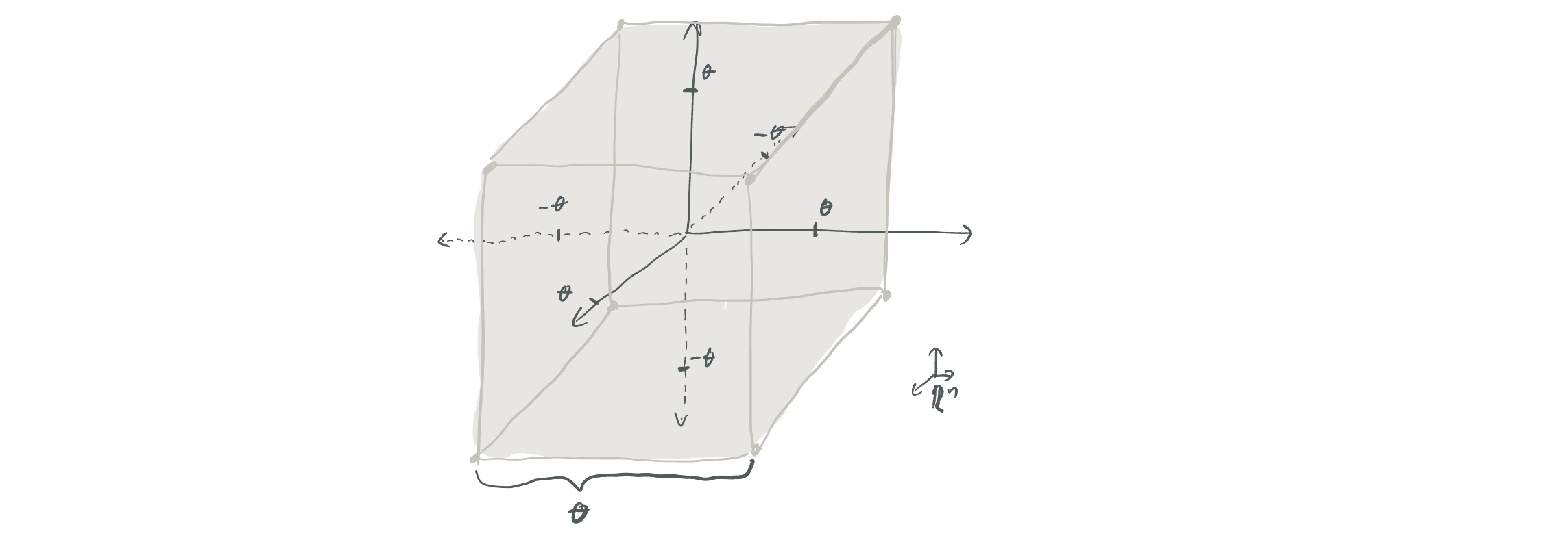
What is \(\theta\)? We set \(\theta\) to ensure that \(\mathbb{E}[\mathsf{Cube}(x)] = 0\), which ends up meaning that \(\theta = \Theta(\sqrt{\log k})\). (Why do we need this expectation to be zero? If it were not close to zero, then \(\mathsf{Cube}\) could be weakly approximated by some constant function, which would immediately make it impossible for the function to be approximately \(d\)-resilient for any \(d\).)

How do we establish the approximate resilience of Cube?

In this part of the post, let \(f^{\leq d}\) represent the components of \(f\) that are correlated with polynomials of degree at most \(d\), and \(f^{> d}\) represent the rest, so \(f(x) = f^{\leq d}(x) + f^{> d}(x)\).

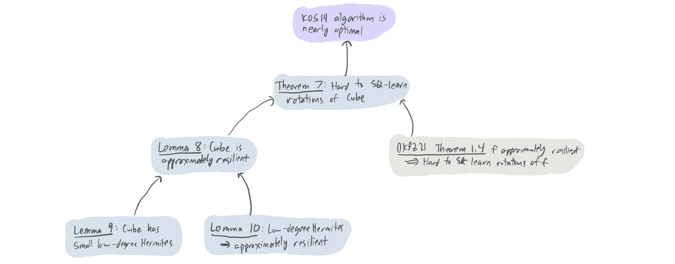
The approximate resilience bound happens in two stages:

[Lemma 9] We show that \(\mathsf{Cube}\) has low degree Hermite coefficients. Put similarly, the total correlation between the function and all low-degree polynomials is small. We concretely show that \(\|\mathsf{Cube}^{\leq d}\|^2 \leq \frac{d}{k} O(\log k)^d\). If we let \(d = c \log(k) / \log\log k\) for sufficiently small \(c\), then \(\|\mathsf{Cube}^{\leq d}\|^2 \leq \frac{1}{k^{0.99}}\).
[Lemma 10] We show that any \(f\) with small low-degree Hermite coefficients is approximately \(d\)-resilient. Concretely, if \(\|f^{\leq d}\|^2 \leq \frac{1}{k^{0.99}}\), then \(f\) is approximately \(\Omega(\log(d) / \log\log d)\)-resilient.

Put together, the two immediately give us a resilience guarantee for \(\mathsf{Cube}\) that mirrors that of \(\mathsf{Tribes}\) from (1) of DFTWW14. This then provides the desired result from (2) of DKPZ21.

The proof of Lemma 9 involves some meticulous analysis of the polynomial coefficients of \(\mathsf{Cube}\), courtesy mainly of Daniel. I’ll refer you to the paper, but this part rests on (1) considering \(\mathsf{Cube}\) as a product of \(k\) interval functions, (2) exactly computing the Hermite coefficients of each interval, and (3) bounding the combined coefficients by some dense summations and applications of Stirling’s inequality.

The proof of Lemma 10 has a little bit of intuition that can likely be conveyed here. We can think about the problem from the lens of function approximation: Can we use \(f\) to create some function \(g\) that is bounded, approximates \(f\), and is uncorrelated with all low-degree polynomials? We’ll make several attempts to convert \(f\) to some \(g\).

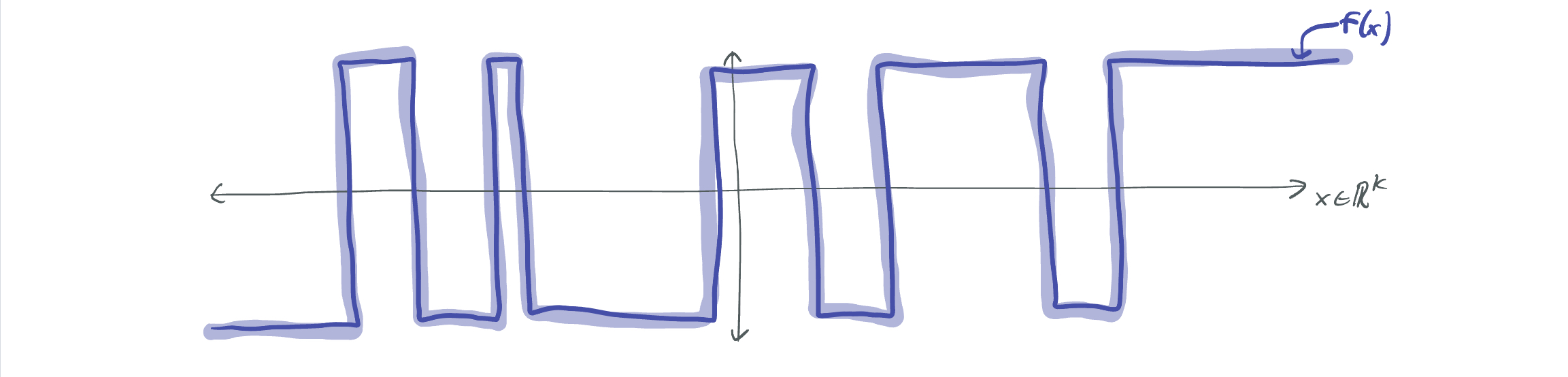
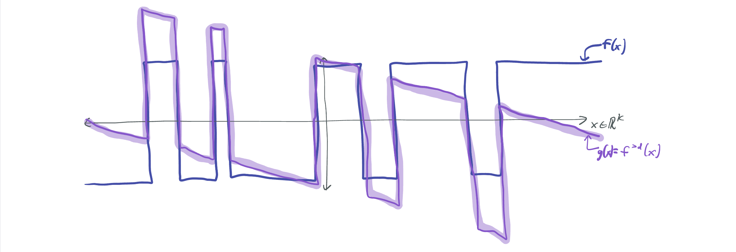
Attempt #1: Drop low-degree polynomials

Let \(g := f^{> d}\). Because \(f\) has small low-degree coefficients, \(g\) closely approximates \(f\). By definition, \(g\) is orthogonal to all polynomials of degree at most \(d\). Yay! But, \(g\) is not a bounded function; as the below image indicates, rotating \(f\) to remove its correlation with a linear function causes \(f\) to approach \(\infty\) (or \(-\infty\)) away from the origin.

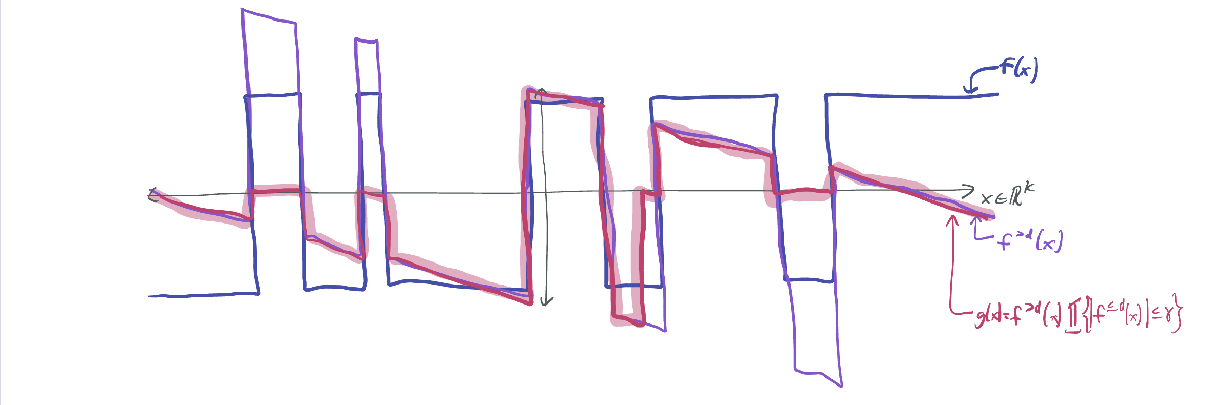
Attempt #2: Drop and threshold

After dropping the low-degree terms, we can re-impose boundedness by setting the function to zero whenever it grows too large: \(g(x) = f^{>d}(x) 1\{\lvert f^{\leq d}(x)\rvert \leq \eta\}\), for some threshold \(\eta > 0\). If \(\eta\) is large, then \(g\) is more similar to \(f\), but could take much larger values. If \(\eta\) is small, then \(g\) cannot be guaranteed to be a good approximation of \(f\), despite its boundedness.

What’s the problem? \(f^{>d}\) may be orthogonal to low-degree polynomials, but multiplying it by this threshold may kill that orthogonality. We gained boundedness, but we lost orthogonality.

Attempt #3: Drop and threshold and drop

What if we just dropped the low-degree terms once again? \(g = [f^{>d} 1\{\lvert f^{\leq d}\rvert \leq \eta\}]^{> d}\). We can use this to restore orthogonality to the previous function. This is precisely what DFTWW14 uses, since they can get a reasonable bound on the maximum value of \(g\), since it’s supported on a finite domain. However, we’re once again faced with the issue that \(g\) loses its boundedness by this additional dropping.

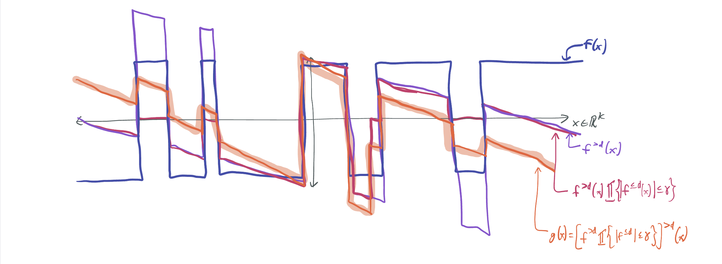
Attempt #4: (Drop and threshold)\(^\infty\)

The previous attempts indicate that if we keep dropping and thresholding the function for carefully chosen thresholds \(\eta\), then we’ll gradually approach an idealized \(g\) that satisfies all of the desired conditions: boundedness, orthogonality, and similarity to \(f\). We do so by defining \(f_0 := f\) and \(f_{i+1} = f_i^{>d} 1\{\lvert f_i^{\leq d}\rvert \leq \eta_i\}\), and letting \(g = \lim_{i \to \infty} f_i\).

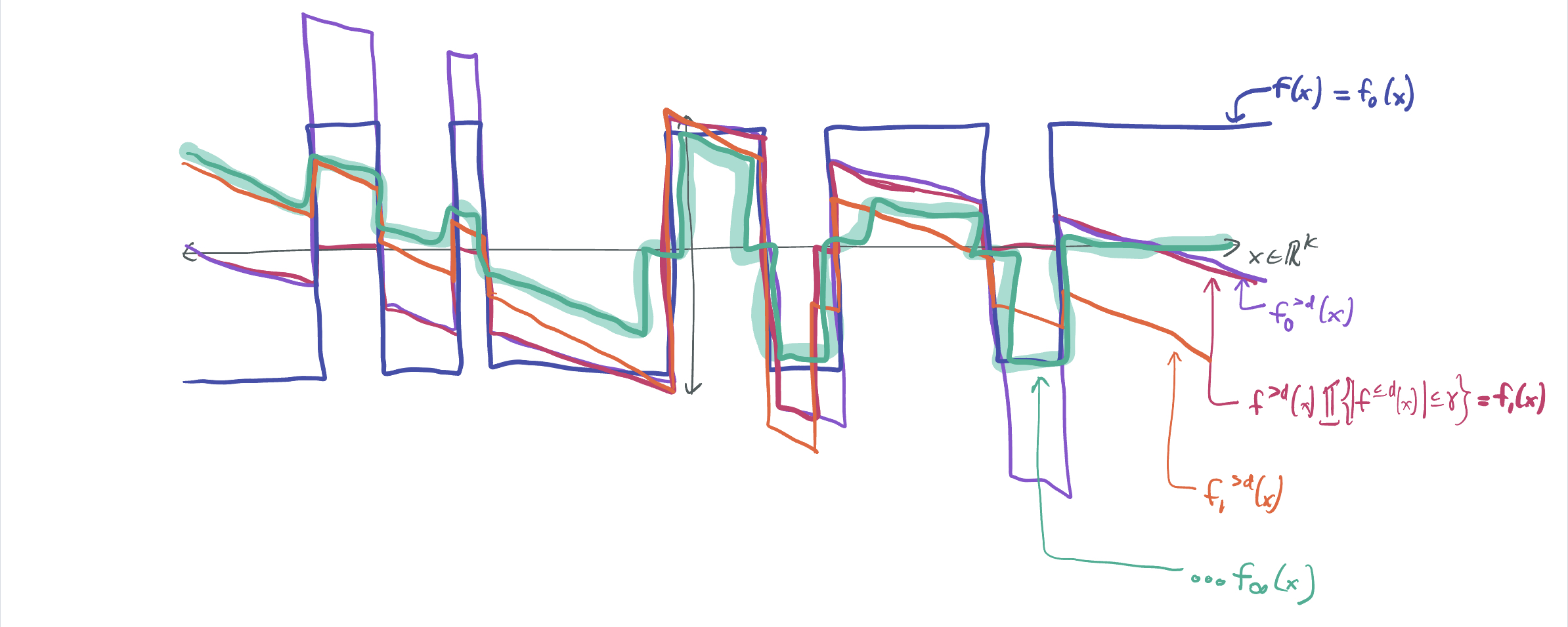
This proof is delicate for 2 reasons:

We need to be careful with our choices of \(\eta_i\), which decrease as \(i\) grows. If they decay too rapidly, then \(g\) might be a very poor approximation of \(f\). Allow \(\eta_i\) to decay too slowly and \(g\) may not end up being bounded. We had to try out a wide range of schedules of \(\eta_i\) before finally finding the right one.
Limits over functions can be tricky, and we ran into several issues when we weren’t precise enough. Fortunately, Manolis is very skilled with this kind of math and we figured out the right way to formalize it.

With this, we got everything we needed: a function \(g\) that validates that \(f\) is approximately resilient as long as its low-degree Hermite coefficients are small. Thus, \(\mathsf{Cube}\) is approximately \(\tilde\Omega(\log k)\)-resilient, and \(\mathcal{H}_k\) cannot be learned with queries of worse tolerance than \(n^{-\tilde\Omega(\log k)}\). This allows us to conclude the optimality of Rocco’s 14-year old algorithm about learning intersections of halfspaces.

Thank you for making it through this monster of a blog post! (Or for scrolling to the bottom of the page.) I really do hope to write more of these, and as always, I’d love any feedback, questions, or ideas.

How hard is it to learn an intersection of halfspaces? (COLT 2022 paper with Rocco, Daniel, and Manolis)