Orthonormal function bases: what they are and why we care
[technical learning-theory background When writing posts on over-parameterized ML models in preparation for my candidacy exam, I realized that many of the theoretical results I discuss rely heavily on orthonormal functions, and that they’ll be difficult for readers to understand without having some background. This post introduces orthonormal families of functions and explains some of the properties that make them convenient mathematical tools. If you want a more thorough (or just plain better) introduction, check out Ryan O’Donnell’s textbook (available for free on his website).
Orthonormality of vectors
For now, forget that I ever said anything about functions being orthonormal. We’ll instead focus on vectors. We define some terms:
- If \(x\) and \(y\) are vectors in \(\mathbb{R}^n\), then \(x\) and \(y\) are orthogonal if they are perpendicular. Mathematically, they’re defined to be orthogonal if \(\langle x, y \rangle = 0\), where \(\langle x, y\rangle = \sum_{i=1}^n x_i y_i\) is the inner product.
- They are orthonormal if they additionally have unit norm: \(\| x \|_2 = \| y \|_2 = 1\), where \(\|x \|_2 = \sqrt{\langle x , x\rangle}\) is the \(\ell_2\) norm.
-
\(u_1, \dots, u_n\) is an orthonormal basis for \(\mathbb{R}^n\) if they are a basis for \(\mathbb{R}^n\) (that is, \(\text{span}(u_1, \dots, u_n) = \mathbb{R}^n\) and they are linearly independent) and if all pairs of vectors are orthonormal. Equivalently, for all \(i, j \in \{1, \dots, n\}\):
\[\langle u_i, u_j \rangle = \delta_{i, j} := \begin{cases} 1 & \text{if } i = j \\ 0 & \text{otherwise.} \end{cases}\]
This basis can be thought of as a rotation of the coordiante axes, since each basis element is perpendicular to every other element.

For example, the above image has an orthonormal basis \(u_1, u_2\) of \(\mathbb{R}^2\). The point \(x\) can be equivalently written as \((x_1, x_2)\) using the standard coordinates axes and as \(\langle x, u_1\rangle u_1 + \langle x, u_2\rangle u_2\) using the rotated axes.
An orthonormal basis \(u_1, \dots, u_n\) of \(\mathbb{R}^n\) is an extremely useful thing to have because it’s easy to to express any vector \(x \in \mathbb{R}^n\) as a linear combination of basis vectors. The fact that \(u_1, \dots, u_n\) is a basis alone guarantees that there exist coefficients \(a_1, \dots, a_n \in \mathbb{R}\) such that \(x = \sum_{i=1}^n a_i u_i\); their orthonormality makes those coefficients easy to compute. Indeed, it simply holds that \(a_i = \langle x, u_i \rangle\) for all \(i\); this can be verified by considering the inner product and applying the orthonormality of the basis elements:
\[\langle x, u_i \rangle = \sum_{j=1}^n a_j \langle u_j, u_i\rangle = \sum_{j=1}^n a_j \delta_{i, j} = a_i.\]This gives rise to some nice properties:
- If we let \(a = (a_1, \dots, a_n) \in \mathbb{R}^n\), then \(\| a\|_2 = \|x \|_2\).
- For some other \(x' \in \mathbb{R}^n\) with \(x'= \sum_{i=1}^n a_i' u_i\), then \(\langle x, x'\rangle = \langle a, a'\rangle\).
- If \(x\) and \(y\) are orthogonal, then \(\|x\|_2^2 + \|y\|_2^2 = \|x + y\|_2^2\). (This is the Pythagorean theorem!)
Generalizing orthonormality to function spaces
These concepts can be generalized beyond simple vector spaces to consider other spaces defined with inner products. If \(\mathcal{X}\) is a Hilbert space with inner product \(\langle \cdot, \cdot \rangle_{\mathcal{X}}\), then we can define \(x, y \in \mathcal{X}\) as orthonormal if \(\langle x, y \rangle_{\mathcal{X}} = 0\) and \(\langle x, x\rangle_{\mathcal{X}} = \langle y, y\rangle_{\mathcal{X}} = 1\).
One important category of Hilbert spaces are \(L_2\) function spaces with distribution \(\mathcal{D}\) over \(\mathcal{X}\). Let \(L_2(\mathcal{D}) = \{f: \mathcal{X} \to \mathbb{R}: \|f\|_{\mathcal{D}} < \infty\}\), where \(\|f\|_{\mathcal{D}} = \sqrt{\mathbb{E}_{x \sim \mathcal{D}} [f(x)^2]}\). This is a Hilbert space with inner-product \(\langle f, g\rangle_{\mathcal{D}} = \mathbb{E}_{x \sim \mathcal{D}}[f(x) g(x)]\) which contains all functions with bounded \(L_2\) norm over this distribution \(\mathcal{D}\). One way to think about this is to think of each function \(f\) as a vector \((f(x))_{x \in \mathcal{X}}\) with infinitely many coordinates and of the inner product as a vector inner product that is weighted by the distribution.
This is a really nice thing to have, because it permits the easy definition of an orthonormal basis for function spaces. This in turn enables functions to be easily represented in terms of other simpler functions, which is useful for all kinds of analysis. We say that \(\mathcal{U} \subseteq L_2(\mathcal{D})\) is an orthonormal basis for \(L_2(\mathcal{D})\) if the following hold:
- \(\mathcal{U}\) spans \(L_2(\mathcal{D})\). That is, for all functions \(f \in L_2(\mathcal{D})\), there exist coefficients \(a_{u} \in \mathbb{R}\) for all \(u \in \mathcal{U}\) such that \(f(x) = \sum_{u \in \mathcal{U}} a_u u(x)\) for all \(x \in \mathcal{X}\).
- The functions in \(\mathcal{U}\) are orthonormal with respect to \(\mathcal{D}\). That is, \(\langle u, u'\rangle_{\mathcal{D}} = \delta_{u, u'}\) for all \(u, u' \in \mathcal{U}\).
These conditions are the same as the conditions for orthonormal bases for vectors, and the properties transition over too!
- For all \(u \in \mathcal{U}\), \(a_u = \langle f, u\rangle_{\mathcal{D}}\).
- \(\|a\|_2 = \sqrt{\sum_{u \in \mathcal{U}} a_u^2} = \|f\|_{\mathcal{D}}\). (This is called the Plancherel theorem.)
- For \(f': \mathcal{X} \to \mathbb{R}\) with \(f' = \sum_{u \in \mathcal{U}} a_u' u\), \(\langle a, a'\rangle = \langle f, f'\rangle_{\mathcal{D}}\). (This is called Parseval’s theorem.)
- If \(\langle f, f'\rangle_{\mathcal{D}} = 0\), then \(\|f\|_{\mathcal{D}}^2 + \|f'\|_{\mathcal{D}}^2 = \|f + f'\|_{\mathcal{D}}^2\).
To explain why this is useful, I introduce several examples of orthonormal bases, which typically come in handy.
Example #1: Parities over the Boolean cube
Let \(\mathcal{X}\) be the \(n\)-dimensional Boolean cube \(\{-1, 1\}^n\) and let \(\mathcal{D}\) be the uniform distribution over the cube. Then, we can write \(\langle f, g\rangle_{\mathcal{D}} = \frac{1}{2^d} \sum_{x \in \{-1, 1\}^n} f(x) g(x)\).
For some \(S\subseteq [n]:= \{1, \dots n\}\), we define a parity function \(\chi_{S}: \{-1, 1\}^n\) to be \(\chi_S(x) = \prod_{i\in S} x_i\). That is, it returns \(1\) if the number of negative coordinates \(x_i\) for \(i \in S\) are even and \(-1\) if they are odd. A parity function is high-frequency if \(|S|\) is large (because flipping a single bit of \(x\) is likely to change the value of \(\chi_S\)) and low-frequency if \(|S|\) is small.
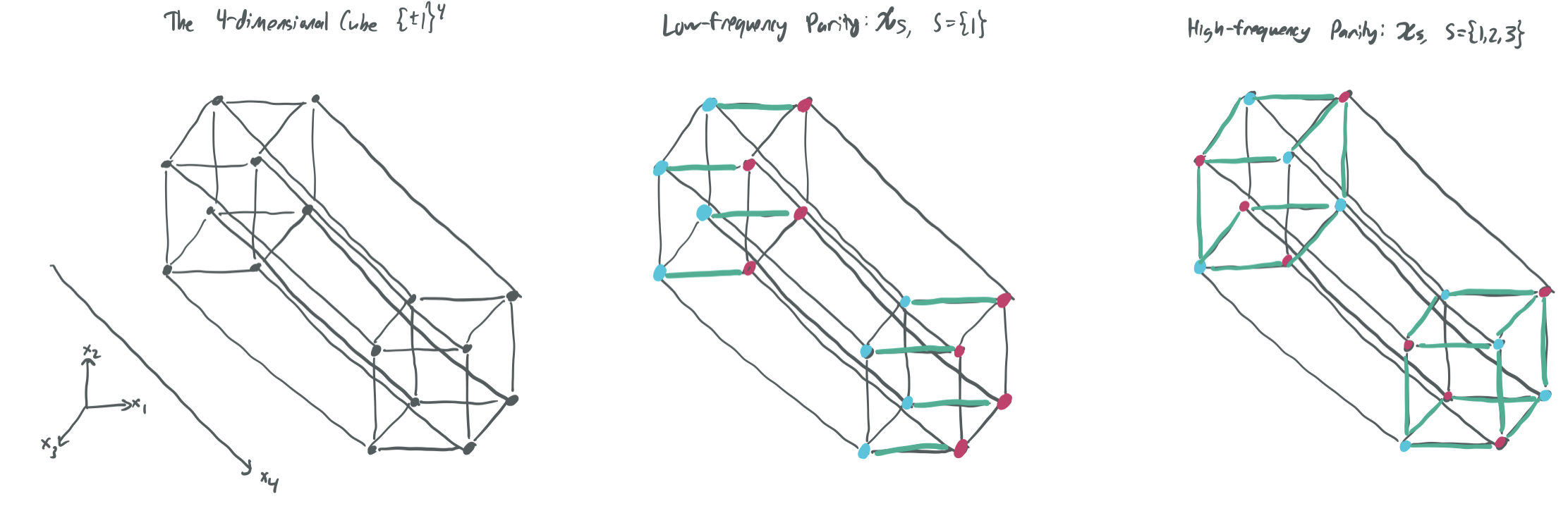
The figure shows two parities defined on \(\{-1, 1\}^4\), one low-frequency and one high-frequency. Note that high-frequency parities change their value much more frequently when moving between adjacent vertices.
The set of all \(2^n\) parity functions \(\{\chi_S: S \subseteq [n]\}\) is an orthonormal basis of \(L_2(\mathcal{D})\), which means that every function \(f\) taking input over the Boolean cube can be expressed as a linear combination of parity functions: \(f = \sum_{S \subseteq [n]} a_S \chi_S\), for \(a_S = \langle f, \chi_S\rangle_{\mathcal{D}}\).
When talking about Fourier expansions (which will be briefly discussed in the next example), functions are thought of as having two equivalent representations:
- The traditional representation, where \(f\) is thought of as a collection of input/output pairs \((x, f(x))\).
- The frequency representation, where \(f\) is thought of as a linear combination of basis elements, which can be parameterized by \((a_S)_{S \subset [n]}\).
Numerous strands of Boolean function analysis rely on dividing a function into high-frequency and low-frequency features, and these equivalent representations are an essential tool towards doing so.
Example #2: Fourier series over the interval
Let \(\mathcal{X} = [-1, 1]\) and let \(\mathcal{D} = \text{Unif}([-1, 1])\). Then, any \(f: [-1, 1] \to \mathbb{R}\) with finite \(\mathbb{E}_{x \sim \text{Unif}([-1, 1])}[f(x)^2]\) be can be expressed as a Fourier series by making use of the following orthonormal basis: \(\mathcal{U} = \{u_j: j \in \mathbb{Z}\}\), for \(u_j(x) = e^{i 2\pi j x}\). (For this example, \(i = \sqrt{-1}\).) These functions are complex-valued, but they still satisfy the conditions necessary for orthonormal bases, which allow functions to be decomposed into high-frequency and low-frequency components.
For people who like trigonometric functions more than complex-valued functions, this basis can be re-written by applying Euler’s formula, \(e^{ix} = \cos(x) + i \sin(x)\):
\[\mathcal{U'} = \{x \mapsto 1\} \cup \{x \mapsto \sqrt{2} \cos(2\pi j x): j \in \mathbb{Z}_+\} \cup\{x \mapsto \sqrt{2} \sin(2\pi j x): j \in \mathbb{Z}_+\}.\]Thus, we can define \(f\) as:
\[f(x) = a_0 + \sum_{j=1}^{\infty}\left(\sqrt{2} a_j \cos(2\pi j x) + \sqrt{2} b_j\sin(2\pi j x) \right)\]for \(a_0 = \langle f, 1\rangle_{\mathcal{D}} = \mathbb{E}_{x}[f(x)]\), \(a_j = \langle f, \sqrt{2} \cos(2\pi j \cdot)\rangle_{\mathcal{D}}\) for \(j \geq 1\), and \(b_j = \langle f, \sqrt{2} \sin(2\pi j \cdot)\rangle_{\mathcal{D}}\).
Again, this gives us a nice decomposition of \(f\) into high- and low-frequency terms. If \(|a_j|\) is large for large values of \(j\), then \(f\) is likely to be “highly bumpy.” Conversely, rapidly decaying values of \(|a_j|\) as \(j\) grows implies that \(f\) will be smooth and closely approximable by low-frequency sines and cosines. Moreover, Plancheral gives us a nice relationship between the norm of the function \(f\) and the size of its coefficients \(a\) and \(b\):
\[\|f\|_{\mathcal{D}}^2 = a_0^2 + \sum_{j=1}^{\infty}(a_j^2 + b_j^2).\]This toolset is really useful for proving facts about functions that satisfy some notion of “smoothness.” My collaborators and I use a generalization of this orthonormal basis in our paper HSSV21 to show that smooth functions (which have bounded Lipschitz constant) can be closely approximated by shallow neural networks with random bottom-layer weights and that some “bumpy” functions with large Lipschitz constants cannot be approximated.
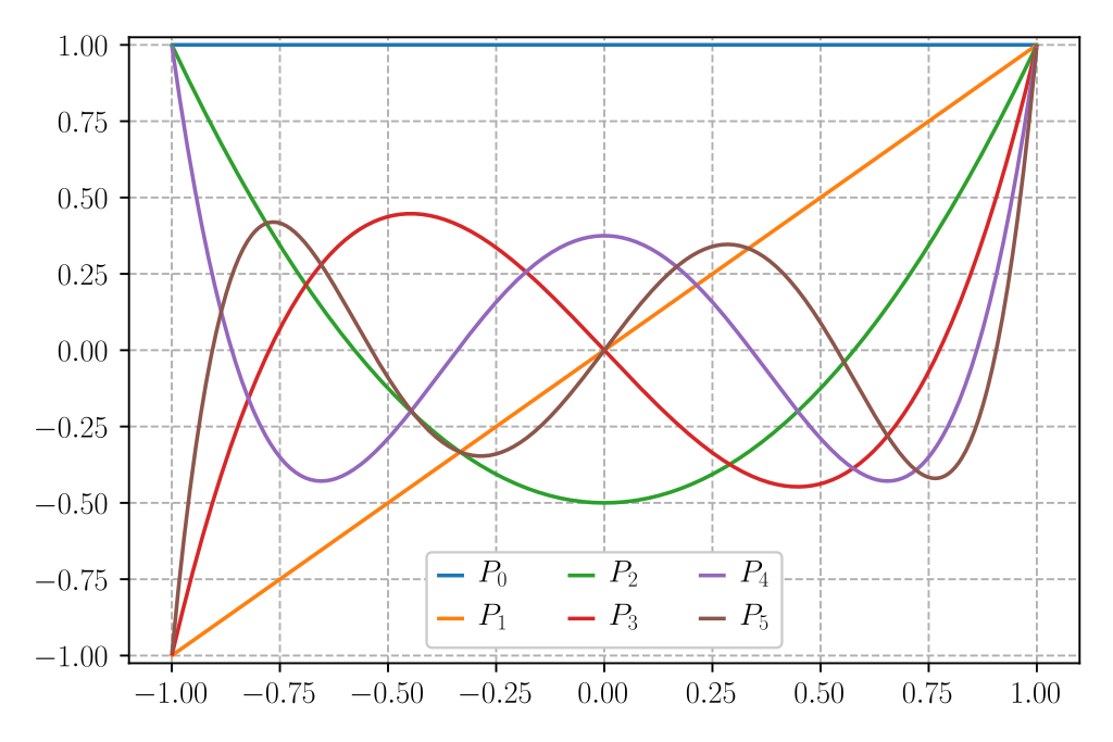
Example #3: Legendre polynomials over the interval
For the same setting as Example #2, there’s another popular orthonormal basis: the Legendre polynomials. Roughly, there are a family of polynomials \(p_0, p_1, \dots\) that are an orthonormal basis for \(L_2(\mathcal{D})\) such that \(p_i\) is a polynomial of degree \(i\). Instead of thinking of decomposing a function over the interval into high- and low-frequency terms, we can now think of the functions as a combination of high- and low-degree polynomials. It’s like a Taylor expansion, except that each Legendre polynomial is uncorrelated to every other Legendre polynomial.
Example #4: Hermite polynomials over Gaussian space
If we instead let \(\mathcal{X} = \mathbb{R}\) and let \(\mathcal{D}\) be the standard normal distribution \(\mathcal{N}(0, 1)\), then the normalized probabilist’s Hermite polynomials are an orthonormal basis for \(L_2(\mathcal{D})\). These again have a nice properties. In particular, each Hermite polynomial \(h_i\) can be defined recursively in terms of \(h_{i-2}\) and \(h_{i-1}\).
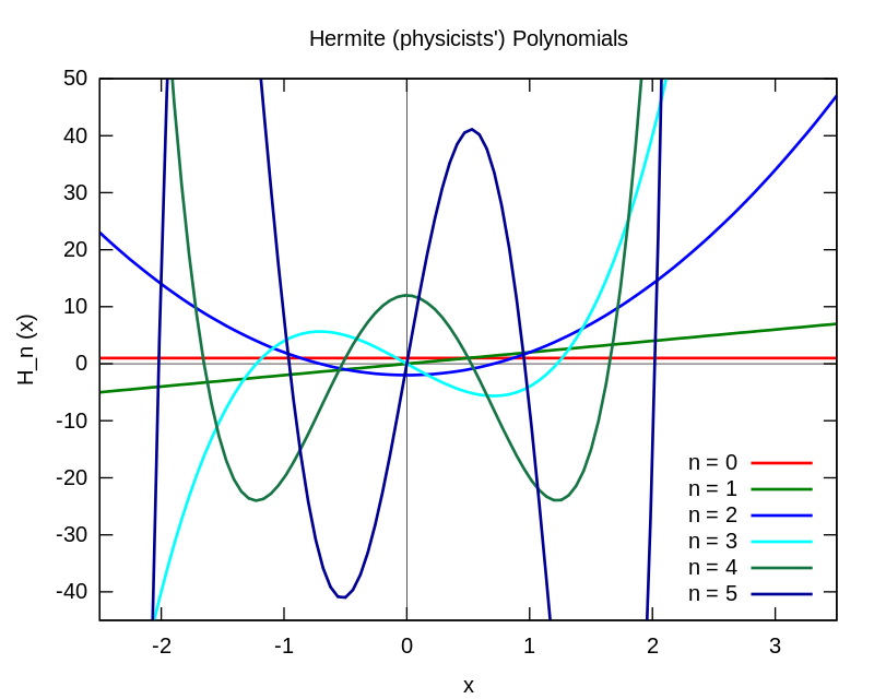
(This and the previous image were shamelessly stolen from the respective Wikipedia articles.)
Comments