[OPML#0] A series of posts on over-parameterized machine learning models
[candidacy technical learning-theory over-parameterized Hello, and welcome to the blog! I’ve been wanting to start this for awhile, and I’ve finally jumped in. This is the introduction to a series of blog posts I’ll be writing over the course of the summer and early in the fall. I hope these posts are informative, and I welcome any feedback on their technical content and writing quality.
I’ve recently finished the second year of my computer science PhD program at Columbia, in which I study the overlap between theoretical comptuer science and machine learning. Over the next few months, I’m going to read a lot of papers about over-parameterized machine learning models—which have a much larger number of parameters than the number of samples. I’ll write summaries of them on the blog, with the goal of making this line of work accessible to people in and out of my research community.
Why am I doing this?
While reading papers is a lot of fun (sometimes), I kind of am required to read this set. CS PhD students at Columbia must take a candidacy exam sometime in their third (or occasionally fourth) year, which requires the student to read 20-25 papers in their subfield in order to better understand what is known and what questions are asked in their research landscape. It culminates with an oral examination, where several faculty members question the student on the papers and future research directions in the subfield.
I’m starting the process of reading the papers now, and I figured that it wouldn’t be such a bad idea to write about what I learn, so that’s what this is going to be.
Why this research area?
Also, what even is an “over-parameterized machine learning model?”
The core motivation of all of my graduate research is to understand why deep learning works so well in practice. For the uninitiated, deep learning is a family of machine learning models that uses complex hierarchical neural networks to represent complicated functions. (If you’re more familiar with theoretical CS than machine learning, you can think of a neural network as a circuit with continuous inputs and outputs.) In the past decade, deep learning has been applied to tasks like object recognition, language translation, and game playing with wild degrees of success. However, the theory of deep learning has lagged far behind these practical successes. This means that we can’t answer simple questions like the following in a mathematically precise way:
- “How well do we expect this trained model to perform on new data?”
- “What are the most important factors in determining how a sample is classified?”
- “How will changing the size of the model affect model performance?”
ML theory researchers have formulated those questions mathematically and produced impressive results about performance guarantees for broad categories of ML models. However, these don’t apply very well to deep learning. In order to get a mathematical understanding of the kinds of questions these researchers ask, I define some terminology about ML models, which I refer back to when describing why theoretical approaches tend to fall short in for deep neural networks.
As a motivating example, consider a prototypical toy machine learning problem: training a classifer that distinguishes images of cats from images of dogs.
- One does so by “learning” a function \(f_\theta: \mathbb{R}^d \to \mathbb{R}\) that takes as input the values of pixels of a photo \(x\) (which we can think of as a \(d\)-dimensional vector) and has the goal of returning \(f_\theta(x) = 1\) if the photo contains a dog and \(f_\theta(x) = -1\) if the photo contains a cat.
-
In particular, if we assume that the pixels \(x\) and labels \(y\) are drawn from some probability distribution \(\mathcal{D}\), then our goal is to find some parameter vector \(\theta \in \mathbb{R}^p\) such that the population error \(\mathbb{E}_{(x, y) \sim \mathcal{D}}[\ell(f_\theta(x), y)]\) is small, where \(\ell: \mathbb{R} \times \mathbb{R} \to \mathbb{R}_+\) is some loss function that we want to minimize. (For instance, the squared loss is \(\ell(\hat{y}, y) = (\hat{y} - y)^2\).)
Notationally, we let \(\mathbb{R}_+\) represent all non-negative real numbers, and \(\mathbb{E}\) be the expectation, where \(\mathbb{E}_{x \sim \mathcal{D}}[g(x)] = \sum_{x} \text{Pr}_{x'\sim \mathcal{D}}[x' = x] g(x).\)
- \(f_\theta\) is parameterized by the \(p\)-dimensional vector \(\theta\), and training the model is the process of choosing a value of \(\theta\) that we expect to perform well and have small population error. In the case of deep learning, \(f_\theta\) is the function produced by computing the output of a neural network with connection weights determined by \(\theta\). In simpler models like linear regression, \(\theta\) directly represents the weights of a linear combination of the inputs: \(f_\theta(x) = \theta^T x\).
- This training process occurs by observing \(n\) training samples \((x_1, y_1), \dots, (x_n, y_n)\) and choosing a set of parameters \(\theta\) such that \(f_\theta(x_i) \approx y_i\) for all \(i= 1, \dots, n\). That is, we find a vector \(\theta\) that yields a small training error \(\frac{1}{n} \sum_{i=1}^n \ell(f_\theta(x_i, y_i))\). The hope is that the learning rule will generalize, meaning that a small training error will lead to a small population error.
This is an over-simplified model that excludes broad categories of ML. It pertains to batch supervised regression problems, where the data provided are labeled, all data is given at once, and the labels are real numbers. While there’s a broad array of topics that we could discuss, we focus on this simple setting in order to motivate the line of research without introducing too much complexity.
Classical learning theory
Over the years, statisticians and ML theorists have studied the conditions necessary for a trained model to perform well on new data. They developed an elegant set of theories to explain when we should expect good performance to occur. The core idea is that more complex models require more data; without enough data, the model will pick up only spurious correlations and noise, learning nothing of value.
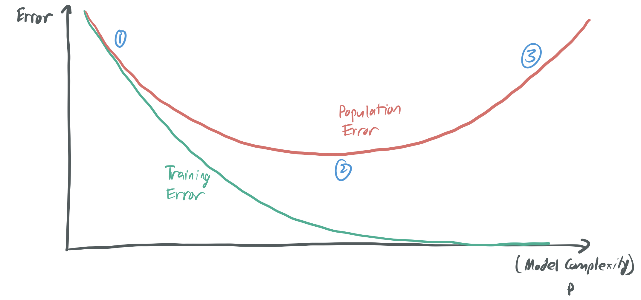
To think about this mathematically, we decompose the population error term into two terms—the training error and the generalization error—and analyze how they change with the model complexity \(p\) and the number of samples \(n\).
\[\underbrace{\mathbb{E}_{(x, y) \sim \mathcal{D}}[\ell(f_\theta(x), y)]}_{\text{population error}} = \underbrace{\frac{1}{n} \sum_{i=1}^n \ell(f_\theta(x_i, y_i))}_{\text{training error}} + \underbrace{\left(\mathbb{E}_{(x, y) \sim \mathcal{D}}[\ell(f_\theta(x), y)] - \frac{1}{n} \sum_{i=1}^n \ell(f_\theta(x_i, y_i)) \right).}_{\text{generalization error}}\]This classical model gives rigorous mathematical bounds that specify when the two components should be small.
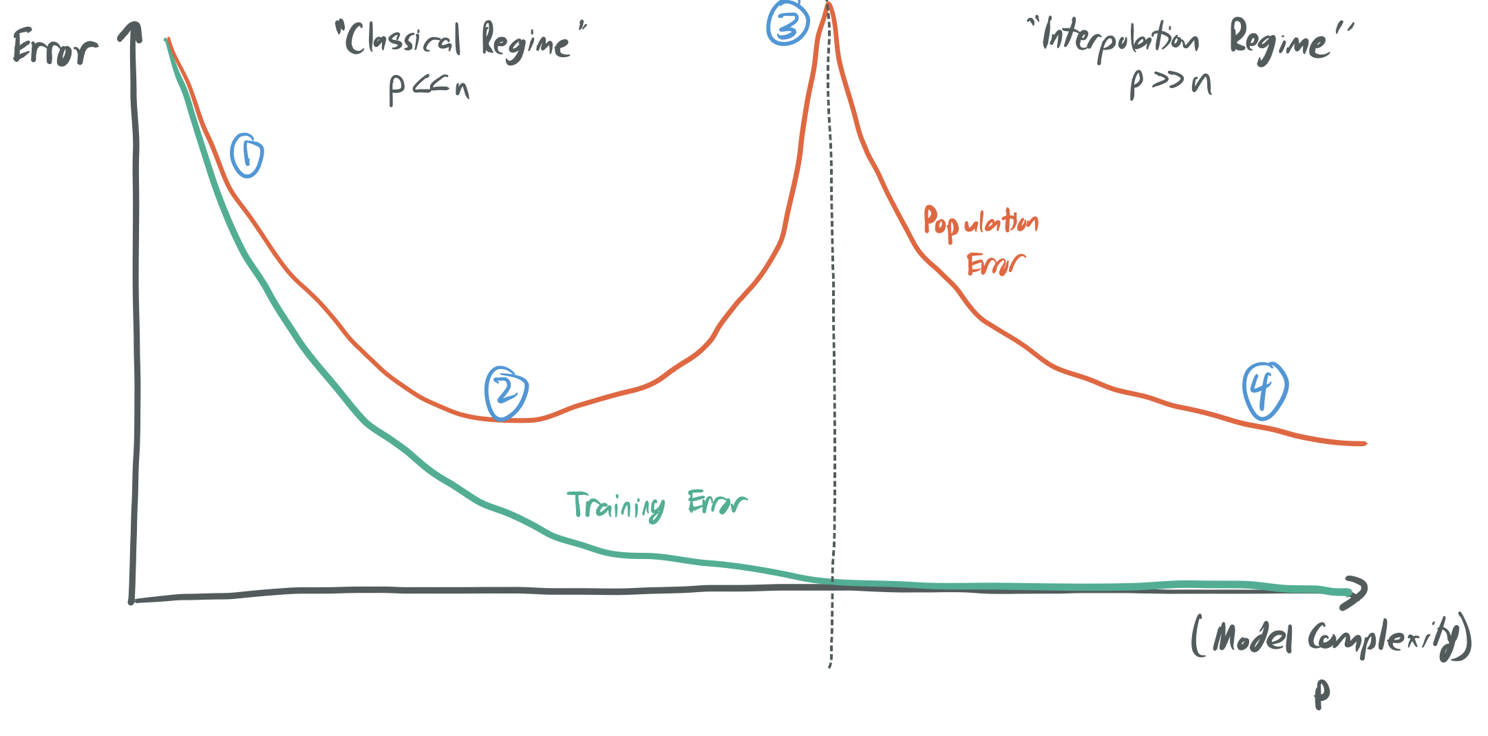
The below image represents the core trade-off that this principle implies; you can find something like it in most ML textbooks.
-
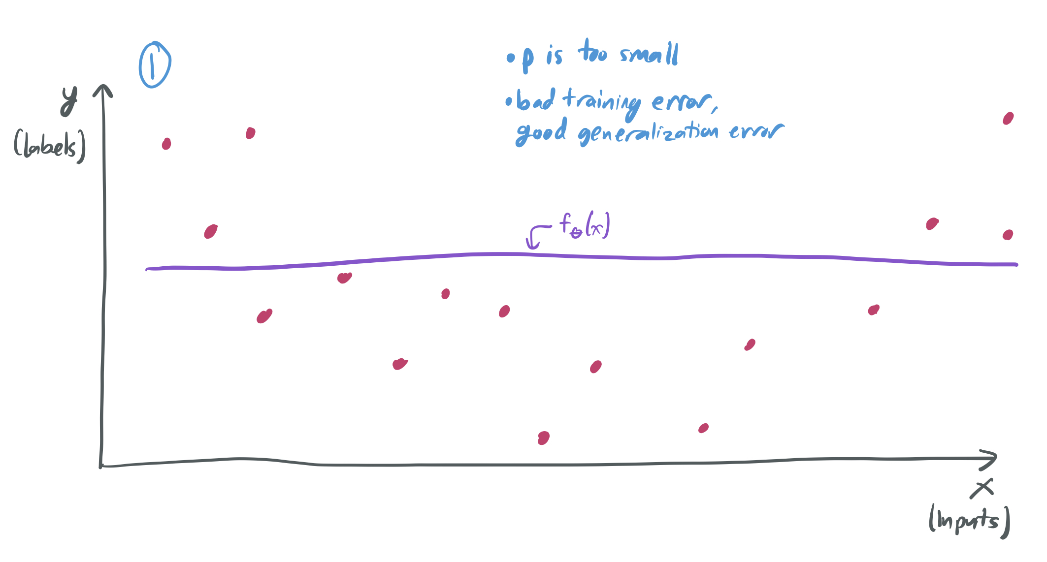
If I choose a very small number of parameters \(p\) relative to the number of samples \(n\), then my model will perform poorly because it’s too simplistic. There will be no function \(f_\theta\) that can classify most of the training data. The training error will be large for any choice of \(\theta\), even though the generalization error is small.
-
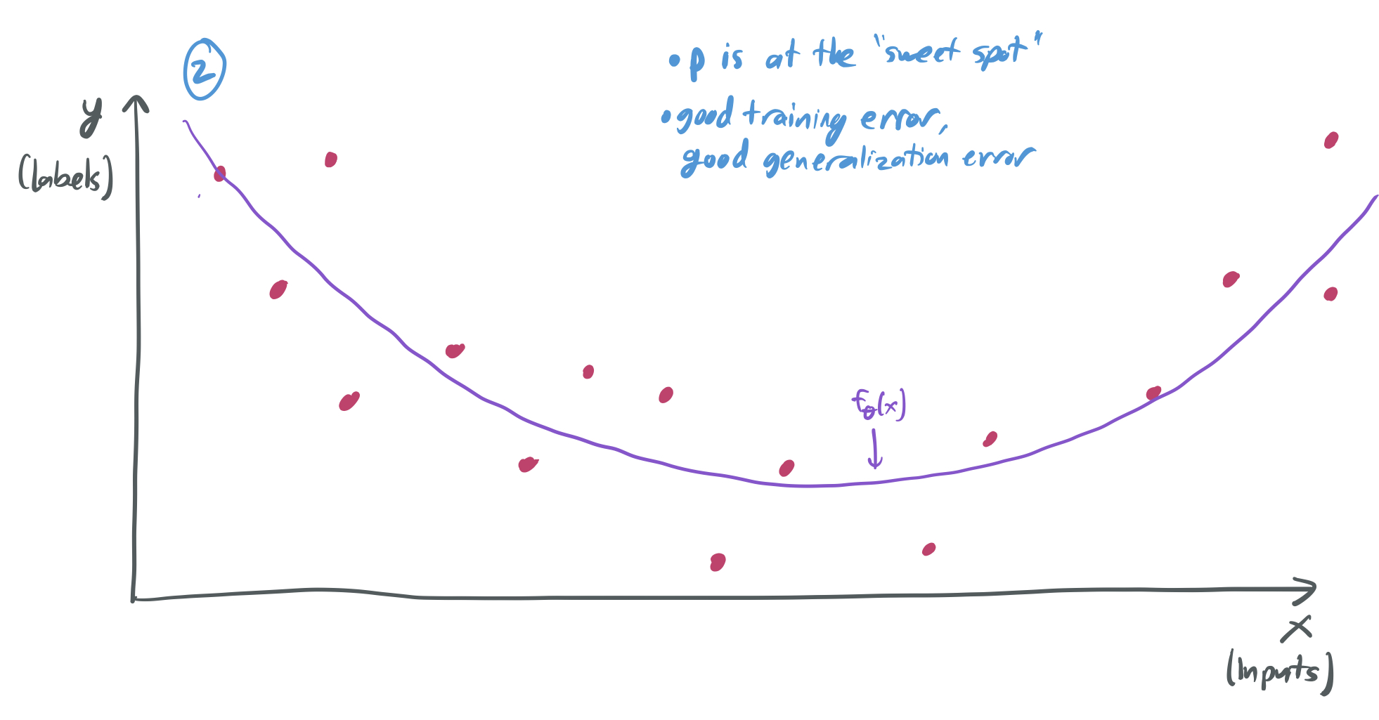
There’s then a “sweet spot” for \(p\), where it’s large enough to capture the complexity of the data distribution, but not too large to overfit. Here, we have a small training error and a generalization error.
-
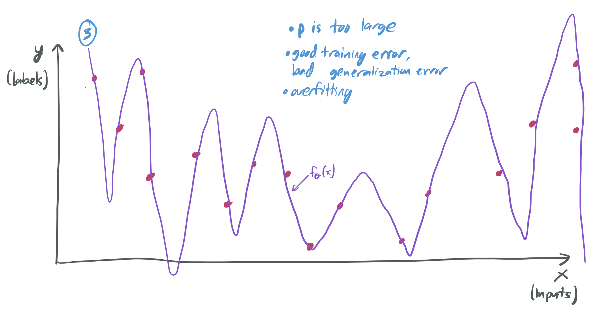
If I choose \(p\) to be large, then I can expect overfitting to occur, where the model has a training error near zero, but the generalization error is very large. In this setting, the model performs poorly because it only memorizes the data, without actually learning the underlying trend.
Classical learning theory offers several tools (like VC-dimension and Rademacher complexity) to quantify the complexity of a model and provide guarantees about how well we expect a model to perform. Based on this theory, over-parameterized models (which have \(p \gg n\)) are expected to be the in the Very Bad second regime, with lots of overfitting and a very large generalization error. However, models of this form often perform much better than this theory anticipates. As a result, there’s a push to develop new theory that better captures what happens when we have more parameters than samples.
The gap between theory and practice
The most prominent case where the classical model fails to explain good performance is for deep learning. Deep neural networks are typically trained with large quantities of data, but they’ll also have more than enough parameters needed to perfectly fit the data; often, there are more parameters than samples. For instance, the state-of-the-art image classifier (as of July 2021) for the standard ImageNet classification task uses roughly 1.8 billion parameters when trained on roughly 14 million training samples, an over-parameterization by a factor of 100. Then, they’re typically trained to obtain zero training error—and purposefully overfit the data—using gradient descent.
Standard approaches to proving generalization bounds provide a bleak picture. For instance:
- The VC-dimension of a neural network with \(p\) different weights, \(L\) layers, and binary output is known to be \(O(p L \log p)\), which implies that it can be learned with \(O(pL \log p)\) samples. This only guarantees success when there are more samples than parameters.
- BFT17 and GRS17 gives generalization error bounds on deep neural networks based on the magnitudes of the weights. However, these bounds grow exponentially with the depth of the network unless the weights are forced to be much smaller than they are in neural networks that succeed in practice.
These approaches give no reason to suspect that the generalization error will be small at all in realistic neural networks with a large number of parameters and unrestricted weights. But neural networks do generalize to new data in practice, which leaves open the question of why that works.
This gap between application and theory indicates that there are more phenomena that are not currently accounted for in our theoretical understanding of deep learning. This also means that much of the practical work in deep learning is not informed at all by theoretical principles. Training neural networks has been dubbed “alchemy” rather than science because the field is built on best practices that were learned by tinkering and is not understood on a first-principles level. Ideally, an explanatory theory of how neural networks work could lead to more informed practice and eventually, more interpretable models.
Over-parameterization and double-descent
This series of posts is (mostly) not about deep learning. Deep neural networks are notoriously difficult to understand mathematically, so most researchers who attempt to do so (including yours truly) must instead study highly simplified variants. For instance, my paper about the approximation capabilities of neural networks with random weights only applies to networks of depth two, because anything else is too complex for our methodology to characterize. So instead of studying deep neural networks, we’ll consider a broader family of ML methods (in particular, linear methods like least-squares regression and support vector machines) when they’re in over-parameterized settings with \(p \gg n\). My hope is that similar principles will explain both the successes of simple over-parameterized models and more complicated deep neural networks.
Broadly, this line of work challenges the famous curve above about the tradeoffs between model complexity and generalization. It does so by suggesting that increasing the complexity of a model (or the number of parameters) can lead to situations where the generalization error decreases once more. This idea is referred to double descent and was popularized by my advisor and his collaborators in papers like BHM18 and BHX19. This augments what is referred to as the classical regime—where \(p \leq n\) and choosing the right model is equivalent to choosing the “sweet spot” for \(p\)—with the interpolation regime. Interpolation means rougly the same thing as overfitting; it describes methods that bring the training loss to zero.
In the interpolation regime, \(p \gg n\) and the learning algorithm selects a hypothesis that perfectly fits the training data (i.e. the training error is zero) and is somehow “smooth,” which leads to some other kind of “simplicity” that then yields a good generalization error. Here’s a way to think about it:
- When \(p \approx n\), it’s likely that there’s exactly one or very few candidate functions \(f_\theta\) that perfectly fit the data, and we have no reason to expect that this function won’t be overly “bumpy” and fail to learn any underlying pattern. (See image (3) above.)
- Instead, if \(p \gg n\), then there will be many hypotheses to choose from that have a training error of zero.
If the algorithm is somehow biased in favor of “smooth” hypotheses, then it’s more likely to pick up on the underlying structure of the data.
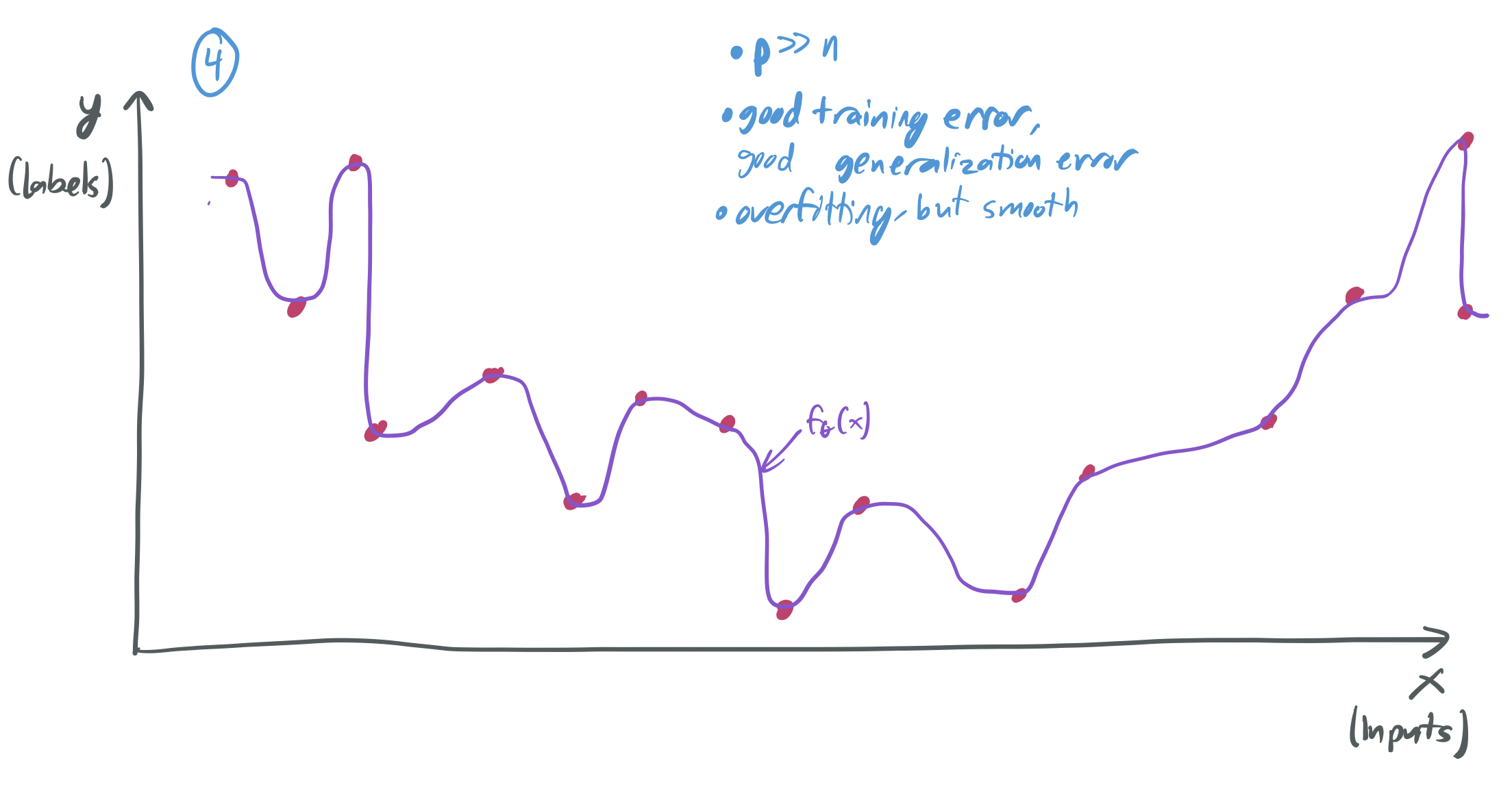
Of course, this is a very hand-wavy way to describe what’s going on. Also, it’s not always the case that having \(p \gg n\) leads to a nice situation like the one in image (4). This kind of success only occurs when the learning algorithm and training distribution meet certain properties. Through this series of posts, I’ll make this more precise and describe the specific mechanisms that enable good generalization in these settings.
What will be covered?
This series aims to have both breadth and depth. I’ll explore a wide range of settings where over-parameterized models perform well and then hone in on linear regression to understand the literature on a very granular level. The following are topics and papers that I’ll read and write about. I’ll add links to the corresponding blog posts once they exist.
This list is subject to change, especially in the next few weeks. If you, the reader, think there’s anything important missing, please let me know!
- Double-descent in linear models:
These papers — which study over-parameterization in the one of the most simple domains possible — will be the main focus of this survey.
- Least-squares regression:
- CD07. Caponnetto and De Vito. “Optimal rates for the regularized least-squares algorithm.” 2007.
- AC10. Audibert and Catoni. “Linear regression through PAC-Bayesian truncation.” 2010.
- WF17. Wang and Fan. “Asymptotics of empirical eigenstructure for high dimensional spiked covariance.” 2017.
- BHX19. [OPML#1]. Belkin, Hsu, and Xu. “Two models of double descent for weak features.” 2019.
- BLLT19. [OPML#2]. Bartlett, Long, Lugosi, and Tsigler. “Benign overfitting in linear regression.” 2019.
- HMRT19. [OPML#4]. Hastie, Montanari, Rosset, and Tibshirani. “Surprises in high-dimensional ridgeless least squares interpolation.” 2019.
- Mit19. Mitra. “Understanding overfitting peaks in generalization error: Analytical risk curves for \(\ell_2\) and \(\ell_1\) penalized interpolation.” 2019.
- MN19. Mahdaviyeh and Naulet. “Risk of the least squares minimum norm estimator under the spike covariance model.” 2019.
- MVSS19. [OPML#3]. Muthukumar, Vodrahalli, Subramanian, and Sahai. “Harmless interpolation of noisy data in regression.” 2019.
- XH19. [OPML#6]. Xu and Hsu. “On the number of variables to use in principal component regression.” 2019.
- BL20. [OPML#5] Bartlett and Long. “Failures of model-dependent generalization bounds for least-norm interpolation.” 2020.
- HHV20. Huang, Hogg, and Villar. “Dimensionality reduction, regularization, and generalization in overparameterized regressions.” 2020.
- Ridge regression:
- Kernel regression:
- Zha05. Zhang. “Learning bounds for kernel regression using effective data dimensionality.” 2005.
- RZ19. Rakhlin and Zhai. “Consistency of Interpolation with Laplace Kernels is a High-Dimensional Phenomenon.” 2019.
- LRZ20. Liang, Rakhlin, and Zhai. “On the multiple descent of minimum-norm interpolants and restricted lower isometry of kernels.” 2020.
- Support Vector Machines:
- MNSBHS20. [OPML#10]. Muthukumar, Narang, Subramanian, Belkin, Hsu, and Sahai. “Classification vs regression in overparameterized regimes: Does the loss function matter?” 2020.
- CL20. [OPML#9]. Chatterji, Long. “Finite-sample Analysis of Interpolating Linear Classifiers in the Overparameterized Regime.” 2020.
- Random feaures models:
- MM19. Mei and Montanari. “The generalization error of random features regression: Precise asymptotics and double descent curve.” 2019.
- Least-squares regression:
- Training beyond zero training error in boosting: While not exactly an over-parameterized model, one well-known example of when training a model past the point of perfectly fitting the data can produce better population errors is with the AdaBoost algorithm. I’ll discuss the original AdaBoost paper and how arguments about the margins of the resulting classifiers suggest that there’s more to training ML models than finding the “sweet spot” discussed above and avoiding overfitting.
- Interpolation of arbitary data in neural networks and kernel machines:
These papers show that both neural networks and kernel machines can interpret data with arbitrary labels and still generalize, even when some fraction of data are noisy.
The former challenges the narrative that classical learning theory that’s oriented around avoiding overfitting can explain deep learning generalization.
The latter suggests that the phenomena are not unique to deep neural networks and that simpler linear models are ripe for study as well.
- ZBHRV17. Zhang, Bengio, Hardt, Recht, and Vinyals. “Understanding deep learning requires rethinking generalization.” 2017.
- BMM18. Belkin, Ma, and Mandal. “To understand deep learning we need to understand kernel learning.” 2018.
- AAK20. Agarwal, Awasthi, Kale. “A Deep Conditioning Treatment of Neural Networks.” 2020.
- Empirical evidence of double descent in deep neural networks:
I’ll survey a variety of papers that relate the above theoretical ideas to experimental results in deep learning.
- BHMM19. Belkin, Hsu, Ma, and Mandal. “Reconciling modern machine-learning practice and the classical bias–variance trade-off.” 2019.
- NKBYBS19. Nakkiran, Kaplun, Bansal, Yang, Barak, and Sutskever. “Deep double descent: Where bigger models and more data hurt.” 2019.
- SGDSBW19. Spigler, Geiger, d’Ascoli, Sagun, Biroli, and Wyart. “A jamming transition from under- to over-parametrization affects generalization in deep learning.” 2019.
- Smoothness of interpolating neural networks as a function of width: Since one of the core benefits of over-parameterized interpolation models is obtaining very smooth functions \(f_\theta\), there’s an interest in understanding how the number of parameters of a neural network can be translated to the smoothnuess of \(f_\theta\). These papers attempt to establish that relationship.
Posts so far
You can also track these under the
- [OPML#0] A series of posts on over-parameterized machine learning models (04 Jul 2021)
- [OPML#1] BHX19: Two models of double descent for weak features (05 Jul 2021)
- [OPML#2] BLLT19: Benign overfitting in linear regression (11 Jul 2021)
- [OPML#3] MVSS19: Harmless interpolation of noisy data in regression (16 Jul 2021)
- [OPML#4] HMRT19: Surprises in high-dimensional ridgeless least squares interpolation (23 Jul 2021)
- [OPML#5] BL20: Failures of model-dependent generalization bounds for least-norm interpolation (30 Jul 2021)
- [OPML#6] XH19: On the number of variables to use in principal component regression (11 Sep 2021)
- [OPML#7] BLN20 & BS21: Smoothness and robustness of neural net interpolators (22 Sep 2021)
- [OPML#8] FS97 & BFLS98: Benign overfitting in boosting (20 Oct 2021)
- [OPML#9] CL20: Finite-sample analysis of interpolating linear classifiers in the overparameterized regime (28 Oct 2021)
- [OPML#10] MNSBHS20: Classification vs regression in overparameterized regimes: Does the loss function matter? (04 Nov 2021)
- My candidacy exam is done! (17 Nov 2021)
What’s next?
This overview post is published alongside the first paper summary about BHX19, which is here. This paper nicely explains how linear regression can perform well in an over-parameterized regime by interpolating the data. It relies on a fairly straight-forward mathematical argument that focuses on a toy model with samples drawn from a nice data distribution, and it’s helpful for seeing the kinds of results that we can expect to prove about models with more parameters than samples. I’ll aim to write a new blog post about a different paper each week until I’m done.
Because research papers are by nature highly technical and because I’m trying to understand them in their full depth, most of these posts will only be accessible to readers with some background in my field. However, I also don’t want to write posts that’ll be useless to anyone who isn’t pursuing a PhD in machine learning theory. My intention is that readers with some amount of background in ML will be able to read them to understand what kinds of questions learning theorists ask; if someone who’s taken an undergraduate-level ML and algorithms course can’t understand what I’m writing, then that’s on me. I’ll periodically give more technical asides into proof techniques that’ll only make sense to people who work directly on research in this area, but I’ll flag them so they’ll be easily skippable.
Maybe this blog will become something more with time… I’m trying to get my feet wet by talking mostly about technical topics that will be primarily of interest to people in my research field, but I may end up branching out to broader subjects that will interest people who aren’t theoretical CS weirdos.
Thanks for making it this far! Hope to see you next time. If I ever get the comments section working, let me know what you think!
Comments