[OPML#1] BHX19: Two models of double descent for weak features
[candidacy technical learning-theory over-parameterized least-squares This is the first of a sequence of blog posts that summarize papers about over-parameterized ML models, which I’m writing to prepare for my candidacy exam. Check out this post to get an overview of the topic and a list of what I’m reading and some notation that I’ll often refer back to.
This week’s summary will cover “Two models of double descent for weak features” by Mikhail Belkin, Daniel Hsu (my advisor!), and Ji Xu (a recently graduated student of Daniel’s), which gives clean examples of when the double-descent phenomenon occurs for linear regression problems. For a high-level overview of double descent, check out the introductory post for this series, which gives a brief summary of the intuition for this phenomenon with some visuals. This paper was released concurrently with BLLT19, HMRT19, and MVSS19, which prove the occurrence of a similar phenomenon with slightly different setups. I’ll write about those two papers for the next two posts, which will cover the more subtle differences between the three papers.
Under certain circumstances, linear regression models with more parameters than samples (“over-parameterized models”) outperform models with fewer parameters. As discussed in the overview post, this flies in the face of classical statistical intuition, where the prevailing idea is that a model can only perform well on never-before-seen samples if the model is simple enough to not overfit the data. They demonstrate this phenomenon for two different regression problems, which they refer to as the Gaussian model and the Fourier model. We’ll focus on the former in this summary.
The contributions of their paper are roughly summarized by the following plot (taken from their Figure 1), which gives the “double-descent” curve that they prove in their setting.
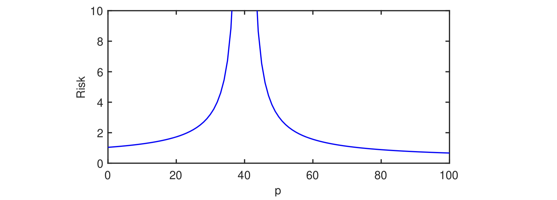 In this example, they consider a setting where \(n = 40\) samples \((x_1, y_1), \dots (x_n, y_n) \in \mathbb{R}^{D} \times \mathbb{R}\) for \(D = 100\) are drawn.
The least-squares linear regression algorithm is used to learn the best linear learning rule using only \(p\) out of \(D\) components of each sample.
As \(p\) increases from 0 to \(n = 40\), the performance of the linear learning rule worsens as the model overfits to the data more dramatically.
This corresponds to the “classical regime” of double-descent, albeit one whose “sweet spot” is at \(p = 0\) and hence never actually experiences the first of the two descents.
In this example, they consider a setting where \(n = 40\) samples \((x_1, y_1), \dots (x_n, y_n) \in \mathbb{R}^{D} \times \mathbb{R}\) for \(D = 100\) are drawn.
The least-squares linear regression algorithm is used to learn the best linear learning rule using only \(p\) out of \(D\) components of each sample.
As \(p\) increases from 0 to \(n = 40\), the performance of the linear learning rule worsens as the model overfits to the data more dramatically.
This corresponds to the “classical regime” of double-descent, albeit one whose “sweet spot” is at \(p = 0\) and hence never actually experiences the first of the two descents.
The strong performance is because of a peculiarity of the data models used by this paper. In more realistic settings, we’d expect that there should be a proper descent in the classical regime. The next section discusses why this model behaves like that.
The interesting behavior occurs when \(p > n\) and the expected risk (which is the mean squared error in this problem setting) of the learning rule improves as \(p\) continues to grow. Here, all of the training samples are able to be perfectly fit by the linear learning rule, and the addition of more features as \(p\) grows beyond \(n\) allows the learning rule to become less volatile and reap the benefits of over-parameterizaton without suffering from the consequences.
This all is very high-level—it’s not clear from the above description how “risk” is defined, how the samples are drawn, and how “volatility” can be quantified. The next section discusses the Gaussian setting in detail and proves that this phenomenon holds in that case.
The Gaussian model
Their model draws labeled samples \((x, y) \in \mathbb{R}^d \times \mathbb{R}\) using the following procedure, for some fixed true parameter vector \(\beta \in \mathbb{R}^d\) and noise parameter \(\sigma > 0\).
- Every component of \(x\) is drawn independently from a standard Gaussian distribution; equivalently, we say that \(x \sim \mathcal{N}(0, I_D)\).
- Noise \(\epsilon\) is drawn from a Gaussian distribution: \(\epsilon \sim \mathcal{N}(0, 1)\).
- The label \(y\) is determined by combining a “ground truth label” \(x^T \beta\) and noise \(\sigma \epsilon\): \(y = x^T \beta + \sigma \epsilon\).
The goal for the learner is to choose some hypothesis parameter vector \(\hat{\beta} \in \mathbb{R}^D\) that has a small expected squared error on unknown data: \(\mathbb{E}_{(x,y)}[( y - x^T \hat{\beta})^2]\). (This is the population loss in this setting.)
So far, we have not discussed the role of \(p\), the number of parameters the learner uses to express \(\hat{\beta}\). This model incorporates \(p\) by giving the learner access to only \(p\) out of \(D\) components of each samples. That is, for some subset \(T \subseteq [D] := \{1, \dots, D\}\) with \(|T| = p\), the learner is given access to samples \(((x_{1, T}, y_1), \dots, (x_{n, T}, y_n)) \in \mathbb{R}^p \times \mathbb{R}\), where \(x_{i,T}\) is a vector of length \(p\) consisting of elements \(x_{i, j}\) where \(j \in T\).
Because the learner does not have access to the the remaining elements \(x_{i, T_c}\), it must come up with the best possible learning rule \(\hat{\beta}\) on the training data that incorporates only those elements. The learning algorithm does so by choosing \(\hat{\beta}_T\) to get the best fit the training inputs to their labels according to the squared error and letting \(\hat{\beta}_{T_c} = 0\). Specifically, the algorithm chooses \(\hat{\beta}_T = X_T^{\dagger} y\) (where \(X_T = [x_{1, T}, \dots, x_{n, T}] \in \mathbb{R}^{n \times p}\), \(y = (y_1, \dots, y_n) \in \mathbb{R}^n\) and \(A^{\dagger}\) is the pseudoinverse of \(A\)), which find the lowest-norm parameter vector that best fits the samples:
- If the training data cannot be perfectly fit (which happens almost always when \(p\leq n\), \(\hat{\beta}_T\) is the parameter vector that best fits the samples: \(\hat{\beta}_T = \arg \min_{\beta_T'} \sum_{i=1}^n (x_{i, T}^T \beta_T' - y_i)^2\).
- Otherwise, if there is some \(\beta_T'\) such that \(X_T \beta_T' = y\) (or \(x_{i, T}^T \beta_T' = y_i\) for all \(i\)), then \(\hat{\beta}_T\) is the parameter vector with minimum norm \(\|\beta_T'\|_2\) of all vectors with that property.
As we’ll see, case (1) corresponds to the “classical regime” (or the left side of the above curve) and case (2) corresponds to the “interpolation regime” (right side).
Based on the definition of the Gaussian model, we describe three settings which we’ll return to later to illustrate how the results work and understand what their limitations are.
- Setting A: All features are equally important. \(\beta = (D^{-1/2}, \dots, D^{-1/2})\) and \(T = [p]\). Here, all of the features have equal weight, so we can expect to only have a \(\frac{p}{D}\) proportion of the “useful information” by seeing \(x_{i, T}\), rather than \(x_i\).
- Setting B: Some features are more important than others, and we have access to the most informative features. \(\beta_j = \frac{c}{j}\) for \(c\) such that \(\|\beta\|_2 = 1\) and \(T = [p]\). Features with low-indices are much more valuable for the learner to have access to than the others, so small values of \(p\) will still provide the learner with useful information.
- Setting C: Some features are more important than others, but we only get a random selection of the features. \(\beta_j = \frac{c}{j}\) such that \(\|\beta\|_2 = 1\) and \(T \subset [D]\) is uniformly drawn from all subsets of size \(p\). While low-index features are more valuable, we can’t guarantee that we’ll have those, so the theoretical guarantees will more closely resemble setting A than setting B.
One of the strange parts of this setting—which we’ll observe when the theoretical results are applied to setting A—is that the “under-parameterized” classical regime never performs well because very little information is provided at all when \(p\) is small. This means that in the eye of the learner, the data is very noisy, because the learner knows nothing about the \(x_{T_c}^T \beta_{T_c} + \sigma \epsilon\) components of \(y\). (\(T_c = [D] \setminus T\) is the complement of \(T\).) As a result, it’s a little bit of an “unfair” setting, where no one can reasonably expect good performance when \(p \ll D\). As is the case with many results in this space, the double-descent phenomenon requires certain peculiarities of the learning models to be studied in order to be cleanly demonstrated.
The main result
Theorem 1 gives exactly the expected risk for the learning rule obtained by using least-squares linear regression on the Gaussian model:
\[\mathbb{E}_{(x, y)}[(y - x^T \hat{\beta})^2] = \begin{cases} (\|\beta_{T_c}\|^2 + \sigma^2) (1 + \frac{p}{n - p - 1}) & \text{if } p \leq n -2;\\ \infty & \text{if } p \in [n-1, n+1]; \\ \|\beta_T\|^2 (1 - \frac{n}{p}) + (\|\beta_{T_c}\|^2 + \sigma^2) (1 + \frac{n}{p - n - 1}) & \text{if } p \geq n+2. \end{cases}\]To make this concrete, we compute the risk for each of the three example settings given above.
-
Setting A: Because the coordinates of \(\beta\) are identical, we can simplify the bound by noting that \(\|\beta_T\|^2 = \frac{p}{D}\) and \(\|\beta_{T_c}\|^2 = 1-\frac{p}{D}\).
\(\mathbb{E}_{(x, y)}[(y - x^T \hat{\beta})^2] = \begin{cases} (1 - \frac{p}{D} + \sigma^2) (1 + \frac{p}{n - p - 1}) & \text{if } p \leq n -2;\\ \infty & \text{if } p \in [n-1, n+1]; \\ (1 - \frac{n}{p} (2 - \frac{D - n - 1}{p - n -1})) + \sigma^2 (1 + \frac{n}{p - n - 1}) & \text{if } p \geq n+2. \end{cases}\) This follows the same pattern as the above plot. As \(p\) increases in size when \(p \leq n - 2\), the second factor diverges to infinity faster than the first term can decrease, leading to the worsening in performance as the model does better at fitting the training data. When \(p \geq n+2\), increasing \(p\) decreases both terms, which gives the descent in the interpolation regime.
-
Setting B: We analyze this setting very roughly, sacrificing precision to explain why a different kind of double-descent curve occurs here. \(\|\beta_{T_c}\|^2\) can be roughly approximated as follows:
\[\|\beta_{T_c}\|^2 = \sum_{j=p+1}^D \frac{c^2}{j^2} \approx \int_{p}^d \frac{c^2}{z^2} dz = -\frac{c^2}{z} \bigg\lvert_{p}^d = \frac{c^2}{p} - \frac{c^2}{d} = \Theta\left(\frac{1}{p}\right).\]Now, we instead get the following risk, expressed in asymptotic notation:
\[\mathbb{E}_{(x, y)}[(y - x^T \hat{\beta})^2] = \begin{cases} \Theta((\frac{1}{p} + \sigma^2) (1 + \frac{p}{n - p - 1})) & \text{if } p \leq n -2;\\ \infty & \text{if } p \in [n-1, n+1]; \\ \Theta((1 - \frac{n}{p}) + (\frac{1}{p} + \sigma^2) (1 + \frac{n}{p - n - 1})) & \text{if } p \geq n+2. \end{cases}\]The authors plot the risk of this curve:
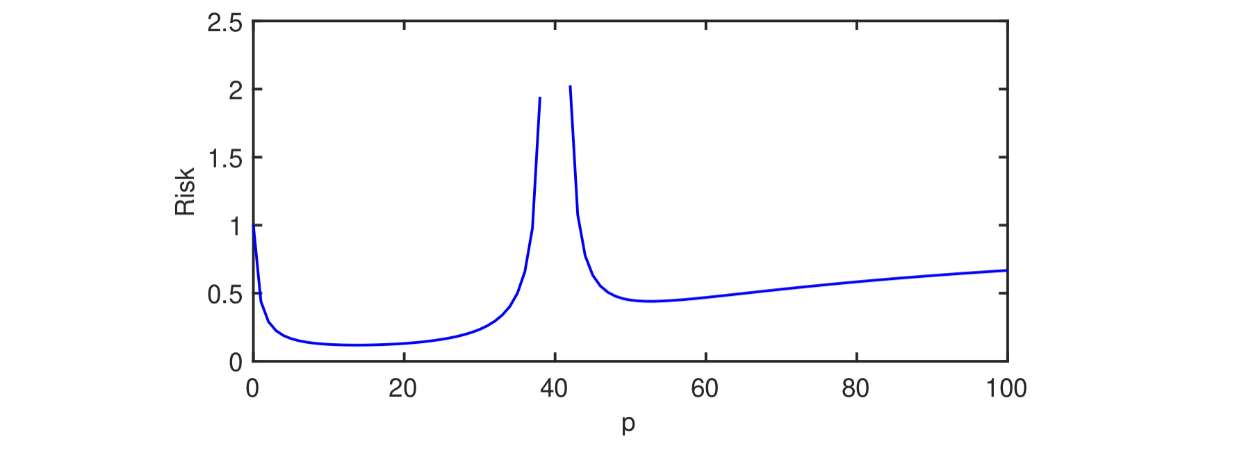
This tells a slightly different story. Because the risk also approaches \(\infty\) as \(p\) approaches zero, there is a now a “sweet spot” where the risk is minimized on the left side of the curve. This resembles a more “traditional” descent curve, where double descent occurs, but where the risk is higher in the interpolation regime. The authors explain that this difference is accounted for by a “scientific” feature selection model, which means that the benefits of interpolation are only fully reaped when the algorithm designer does not have the ability to cherry-pick the most informative features. In other words, it’s possible to obtain good model with few features in the classical regime if we can ensure that the chosen features have more bearing on labels \(y\) than the other features.
-
Setting C: This setting has an identical expected risk to that of Setting A due to the random feature selection, since \(\mathbb{E}[\|\beta_T\|^2] = \frac{p}{D}\). Therefore, the extreme double-descent case detailed in that setting can still occur in cases where different components of \(x\) have orders of magnitude of impact on \(y\) as long as the most informative features cannot be deliberately chosen. This illustrates that the benefits of Setting B can only be reaped when the algorithm designer can “scientifically” choose the best features.
A notable weakness of Theorem 1 is that the results are about the expected squared loss, rather a high-probability guarantee about what the risk will actually be. Theorem 2 offers an improvement by giving concentration bounds on \(\|\beta - \hat{\beta}\|^2\). We won’t go into that in this blog post, but these kinds of bounds will be seen in other papers discussed in future posts.
Proof techniques
The proof of Theorem 1 can be broken down into several manageable steps, which this section will summarize at a high level. This part will be somewhat more jargon-y than the rest of the blog post, so feel free to skim it if it’s not of interest.
Unlike other proofs we’ll see later on, this proof primarily relies on linear algebraic tricks related to orthogonality to exactly compute the expected value of various norms. There is no need for much in the way of probabilistic trickery, because this bound holds in expectation rather than with high probability.
To prove the bound, the expected risk can be partitioned into three distinct terms by expanding the square, plugging in \(y = x^T \beta + \sigma \epsilon\), and noting that \(\hat{\beta}_{T_c} = 0\):
\[\mathbb{E}[(y - x^T \hat{\beta})^2] = \sigma^2 + \|\beta_{T_c}\|^2 + \mathbb{E}[\| \beta_T - \hat{\beta}_T\|^2].\]This tells us that all error for this problem must come from one of three sources, each corresponding to a term: (1) the noisy component of \(y\), \(\sigma \epsilon\); (2) the components of the parameter vector that cannot be determined due to the learner’s ignorance of \(x_{T_c}\), \(\|\beta_{T_c}\|^2\); and (3) the gap between the true parameters and the estimated parameters on the components that the learner is provided, \(\mathbb{E}[\| \beta_T - \hat{\beta}_T\|^2]\).
It suffices to analyze the third term, which can also be written as \(\mathbb{E}[\| \beta_T - X_T^\dagger y\|^2]\). The analysis then splits into two directions: one for the case where \(p \leq n\) and the other for \(p > n\), which is the case because the pseudoinverse \(X_T^\dagger\) is defined as \(X_T^T(X_T X_T^T)^{-1}\) if \(X_T \in \mathbb{R}^{n \times p}\) is a “hot dog” matrix with \(n \leq p\) and \((X_T^T X_T)^{-1} X_T^T\) if \(X_T\) is a “hamburger” matrix with \(n \geq p\).
Note: Because we’re dealing with Gaussian data, we don’t need to worry about issues related to the matrix \(X\) not being full-rank. The \(n\) samples will almost surely span a space of dimension \(n\) if \(n \leq p\) and \(p\) otherwise. If we were drawing samples from a discrete distribution (e.g. uniform from \(\{-1, 1\}^D\), then we’d need to consider the event where the samples are linearly dependent.
We only consider the interpolation case with \(p > n\) here, because the classical case has been well-understood for decades, and the authors refer readers to older works. Given the definition of the pseudoinverse, the difference between the two weight vectors can be decomposed into two terms:
\[\beta_T - \hat{\beta}_T = (I - X_T^T(X_T X_T^T)^{-1}X_T)\beta_T - X_T^T(X_T X_T^T)^{-1} \eta,\]where \(\eta = y - X_T \beta_T\). Note that the two terms must be orthogonal to one another:
- The first term can be written as \(\beta_T - \Pi_T \beta_T\), where \(\Pi_T\) is an orthogonal projection operator onto the rowspace of \(X_T\). Thus, this vector must lie in the null space of \(X_T\).
- The second must lie in the row space of \(X_T\), since it includes a multiplication by \(X_T\).
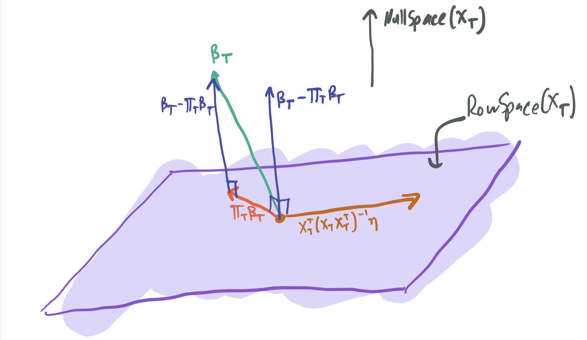
Therefore, the two terms are orthogonal, which means that the Pythagorean theorem can be used to break down the squared norm into two terms:
\[\|\beta_T - \hat{\beta}_T\|^2 = \|\beta_T - \Pi_T \beta_T\|^2 + \|X_T^T(X_T X_T^T)^{-1} \eta\|^2.\]The first term can then be broken up into \(\|\beta_T\|^2 - \|\Pi_T \beta_T\|^2\), again by the Pythagorean Theorem. Applying an expectation, we get \(\mathbb{E}[\|\beta_T\|^2 - \|\Pi_T \beta_T\|^2] = (1 - \frac{n}{p}) \|\beta_T\|^2\).
The second term can be shown to have an expectation of \((\|\beta_{T_c}\|^2 + \sigma^2) \frac{n}{p-n-1}\) by using properties of the Inverse-Wishart distribution.
Plugging these pieces into the initial decomposition of the expected risk gives the theorem.
Fourier series model
The second part of their results in Section 3 focus on a model where the samples \(x\) are rows of a Fourier transform matrix, which are orthogonal to one another. As before, the authors only give a \(p\) out of the \(D\) dimensions of each row to make the model under-specified. They’re similarly able to show a sharp difference between the classical and interpolation regimes, with a risk curve resembling the plot at the beginning of this post. Unlike the Gaussian case, these results hold in the limit, as \(n\), \(p\), and \(D\) all go to infinity, but the ratios \(\rho_n = \frac{n}{D}\) and \(\rho_p = \frac{p}{D}\) are kept fixed.
Future directions / unanswered questions
The key contribution of this paper was to show the existence of a simple setting where the least-squares linear regression algorithm exhibits double-descent and performs best when the number of model parameters is much larger \(p\) than the number samples \(n\). The simplicity of this paper’s setting leaves other questions open about how broad this phenomenon extends beyond these toy examples. The following questions about the generality of the results can be posed:
- Do interpolating models only succeed in “misspecified” settings like this one, where the learner is only given access to a small fraction of the relevant features?
- How do these results extend to data distributions that are not Gaussian? (e.g. what if we instead assume that components of \(x\) have subgaussian tails, or if there can be some dependence between components? What if \(\epsilon\) is not necessarily drawn from a Gaussian distribution?)
- Is there something special about mean squared error, or does this phenomenon also occur when different loss functions are used?
- Will the best results always be found in the classical regime when “scientific feature selection” is used?
Thanks for reading this blog post! If you have any feedback, feel free to comment it below or email me! All feedback is appreciated. Stick around for more on over-parameterization and when it provably works.
Comments