[OPML#2] BLLT19: Benign overfitting in linear regression
[candidacy technical learning-theory over-parameterized least-squares This is the second of a sequence of blog posts that summarize papers about over-parameterized ML models.
This week’s paper is known as BLLT19. Written by Peter Bartlett, Philip Long, Gabor Lugosi, and Alexander Tsigler, this paper is similar to BHX19 [OPML#1] in that both give examples of situations where linear regression models perform better when they have more parameters than samples. However, the two papers study different situations when over-parameterized perform well:
- BHX19 considers a data model where the learner is given only \(p\) out of \(D\) total features and demonstrates that a second descent occurs for expected risk as \(p\) increases beyond \(n\) (the number of samples).
- BLLT19 instead gives the learner access to all of the features and proves bounds on the population error when the model undergoes “benign overfitting.” While they do not strictly give a double-descent curve, they analyze how this benign overfitting can occur when the training data are drawn from a distribution which satisfies certain covariance properties.
Data model
This section introduces a simplified version of their data model and learning algorithm. These simplifications are noted below and make it easier to explain their theoretical results.
- A labeled sample \((x, y) \in \mathbb{R}^p \times \mathbb{R}\) (where \(p\) may be infinite) is drawn as follows:
-
\(x\) is sampled from the multivariate Gaussian distribution \(\mathcal{N}(0, \Sigma)\), where \(\Sigma\) is a diagonal covariance matrix.
Simplification #1: \(\Sigma\) need not be diagonal and \(x\) can instead be drawn from a distribution with subgaussian tails. The paper analyzes the eigenvalues of \(\Sigma\), but since we assume that \(\Sigma\) is diagonal, the eigenvalues are exactly the diagonal entries \(\Sigma_{i,i} = \mathbb{E}[x_i^2] > 0\).
-
There is some true parameter vector \(\theta^* \in \mathbb{R}^p\) with finite norm \(\| \theta^* \|_2 = \sqrt{\sum_{j=1}^p \theta_j^{*2}}\). (This was \(\beta\) in BHX19.)
-
\(y\) is drawn by sampling \(\epsilon\) from a normal distribution \(\mathcal{N}(0, \sigma^2)\) for some \(\sigma > 0\) and letting \(y = x^T \theta^* + \epsilon\).
Simplification #2: \(\epsilon\) is not necessarily Gaussian. Instead, it’s a subgaussian random variable that can depend on \(x\) with a lower-bound on the expectation of its square.
-
-
The learner is provided with \(n\) samples \((x_1, y_1), \dots, (x_n, y_n)\), whose inputs and labels are collected into \(X \in \mathbb{R}^{n \times p}\) and \(y \in\mathbb{R}^n\) respectively.
-
The learner uses the minimum norm estimator (least-squares) \(\hat{\theta}\) to predict \(\theta^*\). This is the same estimator used in BHX19: \(\hat{\theta} = X^T (X X^T)^{-1} y\), which is the vector \(\theta\) minimizing \(\| \theta\|^2\) such that \(X \theta = y\).
Technicality: We can assume that \(X X^T\) is invertible as long as \(p \geq n\). Because they’re drawn from a multivariate Gaussian distribution, \(x_1, \dots, x_n\) will span an \(n\)-dimensional subspace almost surely, which makes \(X\) full-rank.
-
The learner’s prediction \(\hat{\theta}\) is evaluated by the excess risk:
\(R(\hat{\theta}) = \mathbb{E}[(y - x^T \hat{\theta})^2 - (y - x^T \theta^*)^2] = \mathbb{E}[(y - x^T \hat{\theta})^2] - \sigma^2\).
The main object that the authors study is the choice of covariance \(\Sigma\). For simplicity, assume that \(\lambda_i := \Sigma_{i,i}\) for \(1 \leq i \leq p\) and \(\lambda_1 \geq \lambda_2 \geq \dots\). The results depend on how the diagonals of the matrix decay. If the diagonals decay slowly or not at all, then all of the features have a similar impact on the resulting label \(y\). Otherwise, if they decay rapidly, a few features will have an outsized impact on the label. To quantify this decay, they introduce two measurements of the effective rank of \(\Sigma\). For some \(k \in [0, p-1]\), let \(r_{k}(\Sigma) = \frac{\sum_{i > k} \lambda_i}{\lambda_{k+1}}\) and \(R_{k}(\Sigma) = \frac{(\sum_{i > k} \lambda_i)^2}{\sum_{i > k} \lambda_i^2}\). Both terms will be small if the variances rapidly decrease beyond the \((k+1)\)th component of \(x\); they’ll be large if the variances decay slowly or not at all.
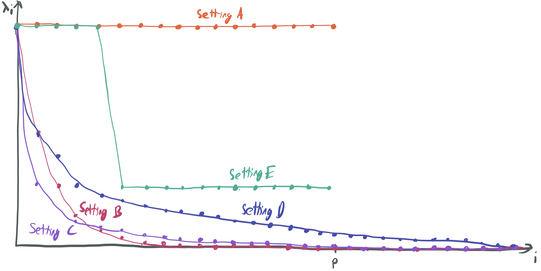
Like in last week’s summary, we introduce several settings with different choices of \(\Sigma\), which we’ll refer back to later when discussing the main result.
- Setting A: Finite features, no decay. Let \(p\) be finite and \(\Sigma = I_p\). Then, \(x\) is isotropic, meaning that all of its components have equal variance. We have \(r_k(\Sigma) = R_k(\Sigma) = p - k\).
- Setting B: Infinite features, rapid decay. Define \(\Sigma\) with \(\lambda_i = \frac{1}{2^i}\). Then, \(r_k(\Sigma) = \frac{1 / 2^k}{1 / 2^{k+1}} = 2\) and \(R_k(\Sigma) = \frac{1 / 4^{k}}{1 / (3 \cdot 4^k)} = 3\).
- Setting C: Infinite features, less rapid decay. Define \(\Sigma\) with \(\lambda_i = \frac{1}{i^2}\). Then, \(r_k(\Sigma) = \frac{\sum_{i=k+1}^\infty i^{-2}}{(k+1)^{-2}} = \frac{\Theta(1/k)}{(k+1)^{-2}} =\Theta(k)\) and \(R_k(\Sigma) = \frac{(\sum_{i=k+1}^\infty i^{-2})^2}{\sum_{i=k+1}^\infty i^{-4}} = \frac{\Theta(1/k^2)}{\Theta(1/k^3)}= \Theta(k)\).
-
Setting D: Infinite features, slow decay. Define \(\Sigma\) with \(\lambda_i = \frac{1}{i \log^2(i+1)}\). By approximating series with integrals, we can roughly compute the sums needed for the effective ranks:
\[\sum_{i > k} \lambda_{k+1} \approx \int_{k}^{\infty} \frac{1}{x \log^2(x)} dx = -\frac{1}{\log x} \bigg\lvert_{k}^{\infty} = \frac{1}{\log k}.\] \[\sum_{i > k} \lambda_{k+1}^2 \approx \int_{k}^{\infty} \frac{1}{x^2 \log^4(x)} dx = \Theta\left(\frac{1}{k \log^4 k}\right).\]Thus, \(r_{k}(\Sigma) = \Theta(k \log k)\) and \(R_{k}(\Sigma) = \Theta(k \log^2 k)\). This is the first case that will give us the kind “benign overfitting” that we’re looking for.
-
Setting E: Finite features, two tiers of importance. Let \(p = n \log n\) and
\[\lambda_i = \begin{cases} 1 & \text{if } i \leq \frac{n}{\log n}, \\ \frac{1}{\log^2(n)} & \text{if } i > \frac{n}{\log n}. \end{cases}\]Then,
\[r_k(\Sigma) = \begin{cases} \Theta\left(\frac{n}{\log n}\right) & \text{if } k < \frac{n}{\log n}, \\ p - k & \text{if } k \geq \frac{n}{\log n}, \\ \end{cases}.\]For \(k \geq \frac{n}{\log n}\), \(R_k(\Sigma) = p-k\) as well.
The main result
This section includes the main upper-bound on risk given by Theorem 4. From this theorem, one can derive sufficient conditions for benign overfitting and non-vacuous error bounds.
First, we define \(k^* = \min\{k \geq 0: r_k(\Sigma) \geq bn\}\) for some constant \(b\). If there is no such \(k\), let \(k^* = \infty\). You can think of this as denoting a separation between “high-impact” and “low-impact” coordinates of \(x\). As stated before, \(r_{k}(\Sigma)\) is small when the variances of coordinates following \(x_{k+1}\) decay rapidly, which means that \(x_{k+1}\) has much larger impact on \(y\) than the following coordinates. Thus, we won’t meet the condition \(r_k(\Sigma) \geq bn\) until there are roughly \(n\) coordinates following \(x_{k+1}\) that have a similar impact on \(y\) to \(x_{k+1}\).
Then, the following bound on risk holds with probability 0.99 over the sample \((x_1, y_1), \dots, (x_n, y_n)\):
\[R(\hat{\theta}) \leq O\left(\|\theta^*\|^2 \lambda_1\left( \sqrt{\frac{r_0(\Sigma)}{n}} + \frac{r_0(\Sigma)}{n}\right) + \sigma^2\left(\frac{k^*}{n} + \frac{n}{R_{k^*}(\Sigma)}\right) \right).\]Simplification #3: The bound is actually shown to hold with probability \(1-\delta\), and hence the right-hand-side also includes \(\log \frac{1}{\delta}\) terms.
To get a sense for what this result means and when it provides a non-vacuous bound, we evaluate it on our five settings. We assume for simplicity that \(\|\theta^*\| = O(1)\) and \(\sigma = O(1)\).
-
Setting A. As long as \(p \geq bn\), \(k^* = 0\). Then, we have that
\[R(\hat{\theta}) \leq O\left(\sqrt{\frac{p}{n}} + \frac{p}{n} + 0 + \frac{n}{p} \right) = O\left(\frac{p}{n}\right).\]Because \(p \geq bn\), this bound is no good, since it does not become small as \(n\) grows. Thus, we cannot guarantee benign overfitting when the components all have equal influence on \(y\). Similarly impactful features lead to a very large effective rank of the entire matrix \(\Sigma\), which blows up the first two terms.
-
Setting B. Because \(r_{k}(\Sigma) = 2\) for all \(k\), there is no choice of \(k\) with \(r_k(\Sigma) \geq bn\) (when \(n\) is large, which it should be) and \(k^* = \infty\). The \(\frac{k^*}{n}\) term renders the bound completely useless.
-
Setting C. In this case, \(k^* = \Theta(n)\) and \(R_{k^*}(\Sigma) = \Theta(n)\). This yields the following risk bound:
\[R(\hat{\theta}) \leq O\left( \sqrt{\frac{1}{n}} + \frac{1}{n} + 1 + 1 \right) = O(1).\]Again, this bound is vacuous, since it does not approach zero as \(n\) increases. Too sharp of a decay in variance of coordinates of \(x\) leads to too large a choice of \(k^*\), which leads the final two terms to not decay to zero. There must be fewer than \(n\) “significant features” to keep the third term from staying large.
-
Setting D. \(k^* = \Theta(n / \log n)\), so \(R_{k^*}(\Sigma) = \Theta(n \log n)\). Plugging this in gives the first non-trivial bound on risk:
\[R(\hat{\theta}) \leq O\left(\sqrt{\frac{1}{n}} + \frac{1}{n} + \frac{1}{\log n} + \frac{1}{\log n} \right) = O\left(\frac{1}{\log n}\right).\]It’s apparent that the bound can guarantee a risk that approaches zero as \(n\) approaches infinity in the infinite-dimensional regime as long as the variances decay just slowly enough to have their sum diverge. (If \(\lambda_i = \frac{1}{i}\), then the \(r_0(\Sigma) = \infty\) because the sum of the diagonals of \(\Sigma\) will diverge.)
Note: Clearly, a rate of \(O(\frac{1}{\log n})\) is not the greatest thing in the world, since it will decay very slowly as \(n\) grows. However, we’re primarily interested in the asymptotic case right now, asking whether the model trends towards zero excess risk as \(n\) becomes arbitrarily large, so this is okay for this context.
-
Setting E. \(k^* = \frac{n}{\log n}\) and \(R_{k^*} = \Theta(n \log n)\). Then,
\[R(\hat{\theta}) \leq O\left(\sqrt{\frac{1}{\log n}} + \frac{1}{\log n} + \frac{1}{\log n} + \frac{1}{\log n} \right) = O\left(\frac{1}{\sqrt{\log n}}\right).\]This gets a somewhat looser bound than Setting D, without requiring infinitely many features.
As illustrated by these examples, this bound imposes several conditions that need to be met for benign overfitting to occur:
- Some of the components of \(x\) must have higher influence than the others, which is necessary to bound the effective rank of the entire matrix \(\Sigma\). That is, we need \(r_0(\Sigma) = \frac{1}{\lambda_1}\sum_{i=1}^p \lambda_i = o(n)\). Setting A fails this condition.
- There must be some separation between “high-impact” and “low-impact” coordinates at \(k^*\), where the low-impact coordinates have high effective rank relative to \(k^*\). For the bound to not be vacuous, we need \(k^* = o(n)\). In other words, there must be a small number of high-impact coordinates followed by a large number of low-impact coordinates of similar importance. Settings B and C have too low an effective rank relative to \(k^*\), \(r_{k^*}(\Sigma)\).
- The other metric of effective rank must be strictly larger than n: \(R_{k^*}(\Sigma) = \omega(n)\). Settings B and C also fail this condition.
The next section discusses how this result is proved and how the above conditions come to be.
Proof techniques for the main result
As was seen in BHX19 last week, the bound on the risk is proved by first decomposing \(R(\hat{\theta})\) into several terms and then bounding each of those terms. Unlike BHX19, this paper’s main result is a bound that holds with high probability, rather than in expectation. As a result, most of the building blocks of this proof will be concentration bounds, which show that certain random variables are very close to their expectations with high probability.
They give the risk decomposition in Lemma 7: With probability \(0.997\) over the training data,
\[R(\hat{\theta}) \leq 2\|\Sigma^{1/2}(I - X^T(XX^T)^{-1}X)\theta^*\|^2 + O(\sigma^2 \text{tr}(C)),\]where and \(C = (XX^T)^{-1} X \Sigma X^T (X X^T)^{-1}\). If the term “bias-variance decomposition” means anything to you, that’s what’s happening here: The first term represents the bias of the best-possible classifier given the data, while the second term corresponds to the variance of the classifier, given the fact that the labels are affected by noise \(\epsilon\).
The proof of this statement occurs in the appendix and is a fairly standard argument, not unlike what was seen in BHX19 last week.
Bias term
Before bounding the bias term, we break it down into more manageable pieces to understand why this corresponds to the bias of the model.
- \(X^T (X X^T) X \theta^*\) is the projection of the true parameter vector \(\theta^* \in \mathbb{R}^p\) onto the span of \(x_1, \dots, x_n \in \mathbb{R}^p\). That is, it’s the linear combination \(v = \sum_{i=1}^n a_i x_i\) minimizing \(\|v - \theta^*\|\).
- \((I - X^T(XX^T)^{-1}X)\theta^*\) then corresponds to \(v - \theta^*\), so this vector has higher magnitude if the projection of \(\theta^*\) onto the span of the rows of \(X\) is far from \(\theta^*\). In general, as \(p\) becomes proportionally larger than \(n\), this vector will become larger because an \(n\)-dimensional subspace will make up a very small subset of \(\mathbb{R}^p\).
- \(\Sigma^{1/2}(I - X^T(XX^T)^{-1}X)\theta^*\) rescales this vector based on the variances of the coordinates. In other words, this transforms down-weights the components of the parameter vector that correspond to “low-impact” coordinates that will be small anyways.
- \(\|\Sigma^{1/2}(I - X^T(XX^T)^{-1}X)\theta^*\|^2\) obtains the squared magnitude of the preceding vector.
Since \(\hat{\theta} = X^T (X X^T)^{-1} y\), it must be the case that \(\hat{\theta}\) lies in the span of the rows of \(X\) as well. Thus, the above quantity is an upper-bound on how closely \(\hat{\theta}\) can correspond to \(\theta^*\) given these restrictions the space where \(\hat{\theta}\) can lie.
Lemma 35 bounds the quantity with probability 0.997 by applying standard concentration bounds with the bounds on the effective rank of \(\Sigma\) captured by \(r_0(\Sigma)\):
\[\|\Sigma^{1/2}(I - X^T(XX^T)^{-1}X)\theta^*\|^2 = O\left( \|\theta^*\|^2 \lambda_1 \left(\sqrt{\frac{r_0(\Sigma)}{n}} + \frac{r_0(\Sigma)}{n} \right) \right).\]Variance term
The matrix \(C = (XX^T)^{-1} X \Sigma X^T (X X^T)^{-1}\) is a bit difficult to make sense of. Roughly, the trace of this matrix will be small when conditions (2) and (3) are met: the existence of many coordinates of \(x\) of comparable variances. In that case, we don’t expect to be hurt much by the noise \(\epsilon\) because it will distribute relatively easily among the comparable coordinates. If they are not comparable, then the effect of the noise cannot “average out” by being dispersed over a lot of similar coordinates. Instead, the noise will dominate the coordinates with low variance, while the coordinates with high variance will not be numerous enough to prevent the noise from corrupting the population of high variance coordinates.
This intuition is encoded by Lemma 11, which bounds its trace with probability 0.997 based on the diagonals of \(\Sigma\):
\[\text{tr}(C) = O\left( \frac{k^*}{n} + \frac{n \sum_{i > k^*} \lambda_i^2}{(\sum_{i > k^*} \lambda_i)^2} \right) = O\left( \frac{k^*}{n} + \frac{n}{R_{k^*}(\Sigma)}\right).\]This is proved by a collection of lemmas that apply concentration bounds to matrix products and facts about eigenvalues.
Proof conclusion
We can put these pieces together by using a union bound. Each of the three inequalities holds with probability 0.997, which means the probability of any of them failing is at most 0.009. Thus, the theorem statement, which comes from combining them, must hold with probability 0.991.
Last thoughts
On a high-level, this paper proves that “benign overfitting” occurs for a narrow sliver of covariance matrices \(\Sigma\), whose variances decay slowly. This complements BHX19, which shows a similar notion of benign overfitting, but instead considers models that exclude components of the data from the learner.
Both models suggest the existence of a large number of weak features is necessary for this phenomenon to occur. BHX19 highlights that “scientific feature selection”—where the highest-impact features are chosen by the learner—negates the need for over-parameterization to have bounded risk. That appears to be true here as well. A large number of weak features are needed for these bounds to hold; however, a “scientific” approach could allow the model to operate well by only using the strong features of their impacts are known a priori.
Next time, I’ll write about MVSS19, which is another similar paper that proves similar statements to BLLT19, but from a somewhat different angle that focuses on describing an intuition for why the variances must decay in a particular way. Put together, the three papers characterize a range of peculiar instances (e.g. misspecified data, slowly decaying components) where an over-parameterized approach does better than the classical literature suggests.
Comments