How many neurons are needed to approximate smooth functions? A summary of our COLT 2021 paper
[technical research neural-net learning-theory In the past few weeks, I’ve written several summaries of others’ work on machine learning theory. For the first time on this blog, I’ll discuss a paper I wrote, which was a collaboration with my advisors, Rocco Servedio and Daniel Hsu, and another Columbia PhD student, Manolis Vlatakis-Gkaragkounis. It will be presented this week at COLT (Conference on Learning Theory) 2021, which is happening in-person in Boulder, Colorado. I’ll be there to discuss the paper and learn more about other work in ML theory. (Hopefully, I’ll put up another blog post after about what I learned from my first conference.)
The paper centers on a question about neural network approximability; namely, how wide does a shallow neural network need to be to closely approximate certain kinds of “nice” functions? This post discusses what we prove in the paper, how it compares to previous work, why anyone might care about this result, and why our claims are true. The post is not mathematically rigorous, and it gives only a high-level idea about why our proofs work, focusing more on pretty pictures and intuition than the nuts and bolts of the argument.
If this interests you, you can check out the paper to learn more about the ins and outs of our work. There are also two talks—a 90-second teaser and a 15-minute full talk—and a comment thread available on the COLT website. This blog post somewhat mirrors the longer talk, but the post is a little more informal and a little more in-depth.
On a personal level, this is my first published computer science paper, and the first paper where I consider myself the primary contributor to all parts of the results. I’d love to hear what you think about this—questions, feedback, possible next steps, rants, anything.
I. What’s this paper about?
A. Broad background on neural nets and deep learning
As I discuss in the overview post for my series on over-parameterized ML models, the practical success of deep learning is poorly understood from a mathematical perspective. Trained neural networks exhibit incredible performance on tasks like image recognition, text generation, and protein folding analysis, but there is no comprehensive theory of why their performance is so good. I often think about three different kinds of questions about neural network performance that need to be answered. I’ll discuss them briefly below, even if only only the first question (approximation) is relevant to the paper at hand.
-
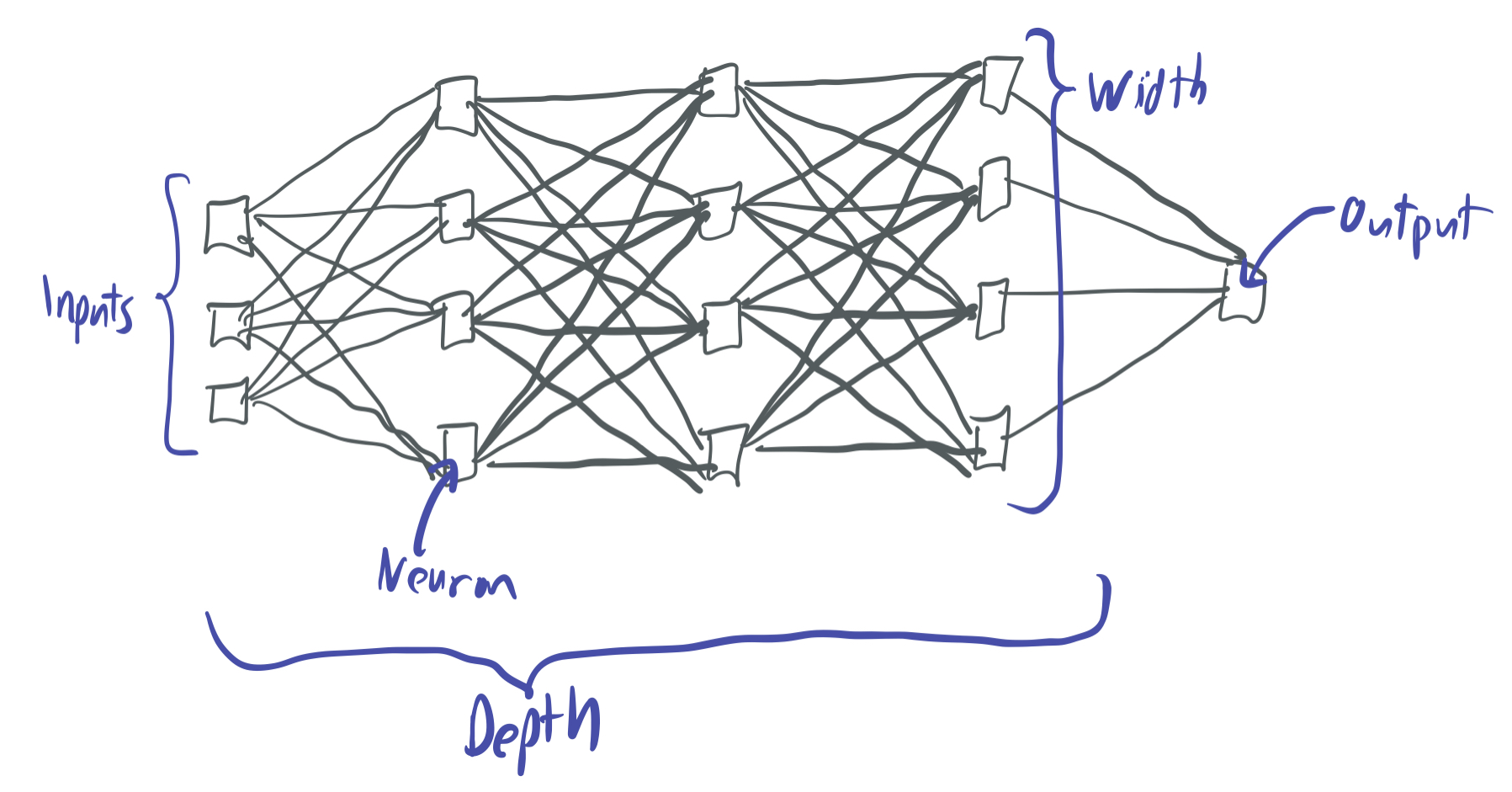
Approximation: A neural network is a type of mathematical function that can be represented as a hierarchical arrangement of artifical neurons, each of which takes as input the output of previous neurons, combines them together, and returns a new signal. These neurons are typically arranged in layers, where the number of neurons per layer is referred to as the width and the number of layers is the depth.
Mathematically, each neuron is a function of the outputs of neurons in a previous layer. If we let \(x_1,x_2, \dots, x_r \in \mathbb{R}\) be the outputs of the \(L\)th layer, then we can define a neuron in the \((L+1)\)th layer as \(\sigma(b + \sum_{i=1}^r w_i x_i)\) where \(b \in \mathbb{R}\) is a bias, \(w \in \mathbb{R}^r\) is a weight vector, and \(\sigma: \mathbb{R} \to \mathbb{R}\) is a nonlinear activation function. If the parameters \(w\) and \(b\) are carefully selected for every neuron, then many layers of these neurons allow for the representation of complex prediction rules.
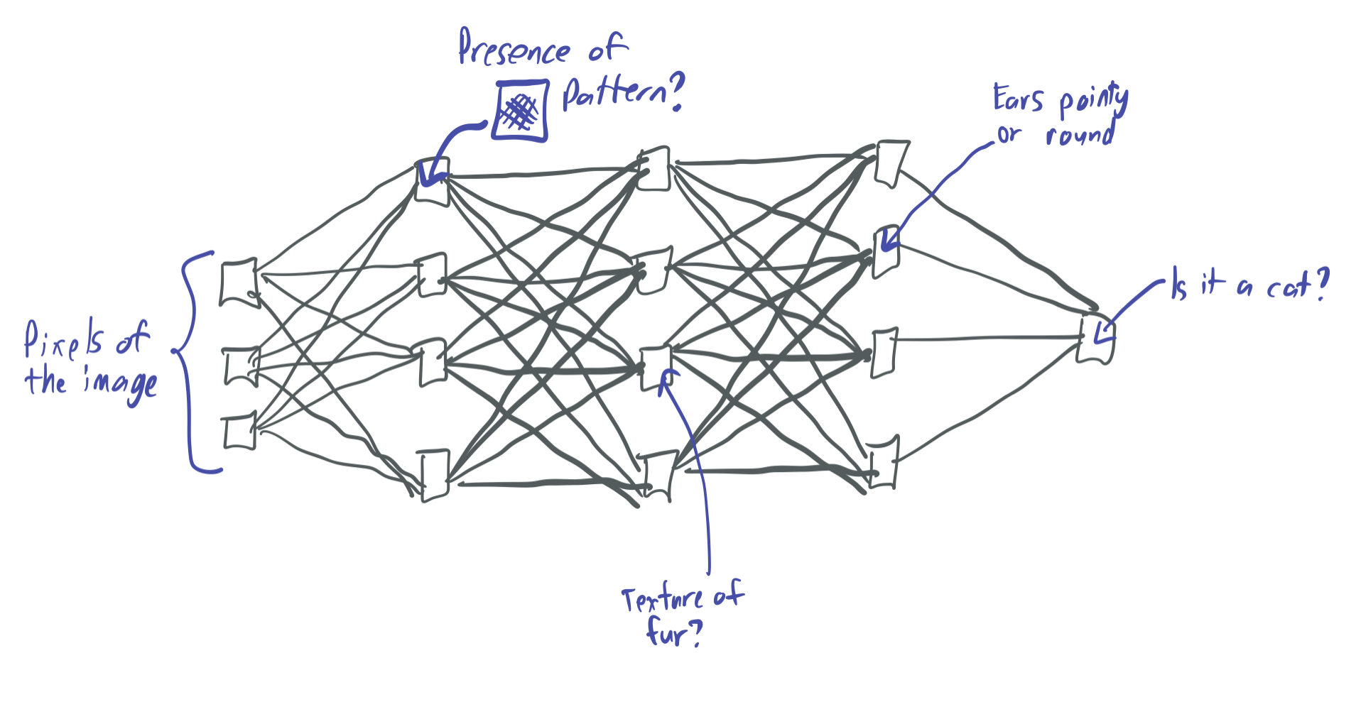
For instance, if I wanted a neural network to distinguish photos of cats from dogs, the neural network would represent a function mapping the pixels from the input image (which can be viewed as a vector) to a number that is 1 if the image contains a dog and -1 if the image has a cat. Typically, each neuron will correspond to some kind of visual signal, arranged hierarchically based on the complexity of the signal. For instance, a low-level neuron might detect whether a region of the image contains parallel lines. A mid-level neuron may correspond to certain kind of fur texture, and a high-level neuron could identify whether the ears are a certain shape.
This opens up questions about the expressive properties of neural networks: What kinds of functions can they represent and what kinds can’t they? Does there have to be some kind of “niceness” property of the “pixels to cat” map in order for it to be expressed by a neural network? And how large does the neural network need to be in order to express some kind of function? How does increasing the width increase the expressive powers of the network? How about the depth?
This paper asks questions like these about a certain family of shallow neural networks. We focus on abstract mathematical functions—there will be no cats or dogs here—but we believe that this kind of work will better help us understand why neural networks work as well as they do.
-
Optimization: Just because there exists a neural network that can represent the prediction rule you want doesn’t mean it’s possible to algorithmically find that function. The \(w\) and \(b\) parameters for each neuron cannot be feasibly hard-coded by a programmer due to the complexity of these kinds of functions. Therefore, we instead learn the parameters by making use of training data.
To do so, a neural network is initialized with random parameter choices. Then, given \(n\) training samples (in our case, labeled images of cats and dogs), the network tunes the parameters in order to come up with a function that predicts correctly on all of the samples. This procedure involves using an optimization algorithm like gradient descent (GD) or stochastic gradient descent (SGD) to tune a good collection of parameters.
However, there’s no guarantee that such an algorithm be able to find the right parameter settings. GD and SGD work great in practice, but they’re only guaranteed to work for a small subset of optimization problems, such as convex problems. The training loss of neural networks is non-convex and isn’t one of the problems that can be provably solved with GD or SGD; thus, there’s no guarantee of convergence here.
There’s lots of interesting work on optimization, but I don’t really go into it in this blog.
-
Generalization: I’ll be brief about this, since I discuss it a lot more in my series on over-parameterized ML models. Essentially, it’s one thing to come up with a function that can correctly predict the labels of fixed training samples, but it’s another entirely to expect the prediction rule to generalize to new data that hasn’t been seen before.
The ML theory literature has studied the problem of generalization extensively, but most of the theory about this focuses on simple settings, where the number of parameters \(p\) is much smaller than the number of samples \(n\). Neural networks often live in the opposite regime; these complex and hierarchical functions often have \(p \gg n\), which means that classical statistical approaches to generalization don’t predict that neural networks will perform well.
Many papers have tried to explain why over-parameterized models exceed expectations in practice, and I discuss some of those in my other series. But again, this paper does not go into this.
B. More specific context on approximation
As mentioned above, this paper (and hence this post) focuses on the first question of approximation. In particular, it discusses the representational power of a certain family of shallow neural networks. (Typically, “shallow” means depth-2—or one-hidden layer—and “deep” means any networks of depth 3 or more.)
There’s a well-known result about depth-2 networks that we build on: The Universal Approximation Theorem, which states that for any continuous function \(f\), there exists some depth-2 network \(g\) that closely approximates \(f\). (We’ll define “closely approximates” later on.) Three variants of this result were proved in 1989 by three different papers. Here’s a blog post that gives a nice explanation of why these universal approximation results are true.
At first glance, it seems like this would close the question of approximation entirely; if a depth-2 neural network can express any kind of function, then there would be no need to question whether some networks have more approximation powers than others. However, the catch is that the Universal Approximation Theorem does not guarantee that \(g\) will be of a reasonable size; \(g\) could be an arbitrarily wide neural network, which obviously is a no-go in the real world where neural networks actually need to be computed and stored.
As a result, many follow-up papers have focused on the question about which kinds of functions can be efficiently approximated by certain neural networks and which ones cannot. By “efficient,” we mean that we want to show that a function can be approximated by a neural network with a size polynomial in the relevant parameters (the complexity of the function, the desired accuracy, the dimension of the inputs). We specifically do not want a function that requires size exponential in any of these quantities.
Depth-separation is an area of study that has focused on studying the limitations of shallow networks compared to deep networks.
- A 2016 paper by Telgarsky shows that there exist some very “bumpy” triangular functions that can be approximated by neural networks of depth \(O(k^3)\) with polynomial-wdith, but which require exponential width in order to be approximated by networks of depth \(\Omega(k)\).
- Papers by Eldan and Shamir (2016), Safran and Shamir (2016), and Daniely (2017) exhibit functions that separate depth-2 from depth-3. That is, the functions can be approximated by polynomial-size depth-3 networks, but they require exponential width in order to be approximated by depth-2 networks.
One thing that these papers have in common is that they all require one of two things. Either (1) the function is a very “bumpy” one that is highly oscillatory, or (2) the depth-2 networks can partially approximate the function, but cannot approximate it to an extremely high degree of accuracy. A 2019 paper by Safran, Eldan, and Shamir noticed this and asked whether there exist “smooth” functions that have separation between depth-2 and depth-3. This question was inspirational for our work, which poses questions about the limitations of certain kinds of 2-layer neural networks.
C. Random bottom-layer ReLU networks
We actually consider a slightly more restrictive model than depth-2 neural networks. We focus on two-layer random bottom-layer (RBL) ReLU neural networks. Let’s break that down into pieces:
-
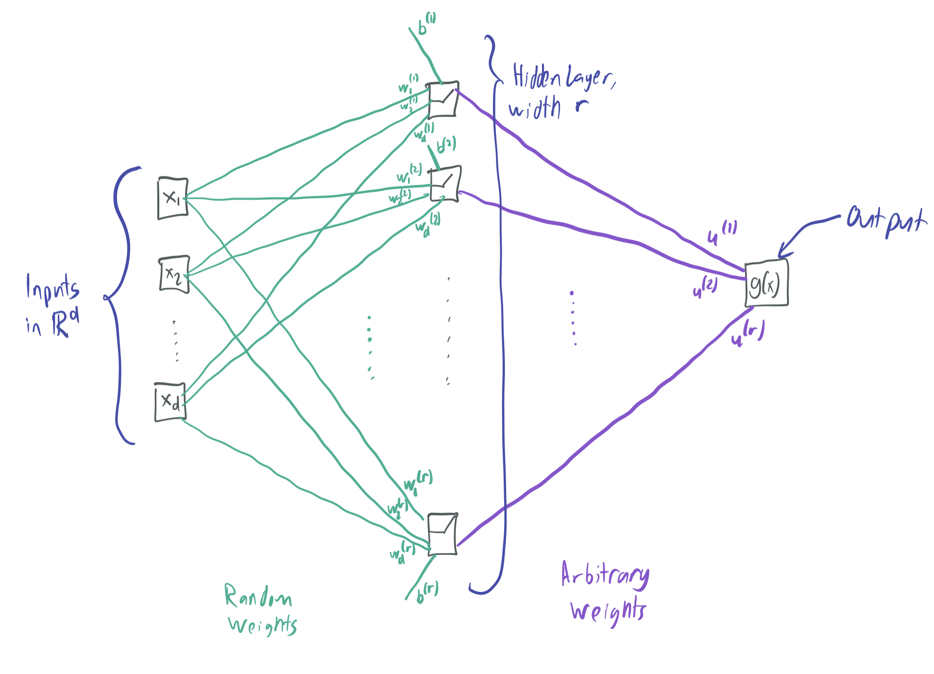
“two layer” means that the neural network has a single hidden layer and can be represented by the following function, for parameters \(u \in \mathbb{R}^r, b \in \mathbb{R}^{r}, w \in \mathbb{R}^{r \times d}\):
\[g(x) = \sum_{i=1}^r u^{(i)} \sigma(\langle w^{(i)}, x\rangle + b^{(i)}).\]\(r\) is the width of the network and \(d\) is the input dimension.
- “random bottom-layer” means that \(w\) and \(b\) are randomly chosen and then fixed. That means that when trying to approximate a function, we can only tune \(u\). This is also called the random feature model in other papers.
- “ReLU” refers to the restricted linear unit activation function, \(\sigma(z) = \max(0, z)\). This is a popular activation function in deep learning.
The following graphic visually summarizes the neural network:
Why do we focus on this family of neural networks?
- Any positive approximation results about this model also apply to arbitrary networks of depth 2. That is, if we want to show that a function can be efficiently approximated by a depth-2 ReLU network, it suffices to show that it can be efficiently approximated by a depth-2 RBL ReLU network. (This does not hold the other direction; there exist functions that can be efficiently approximated by depth-2 ReLU networks that cannot be approximated by depth-2 RBL ReLU nets.)
- According to papers like Rahimi and Recht (2008), kernel functions can be approximated with random feature models. This means that our result can also be used to comment on the approximation powers of kernels, which Daniel discusses here.
- Recent research on the neural tangent kernel (NTK) studies the optimization and generalization powers of randomly-initialized neural networks that do not stray far from their initialization during training. The question of optimizing two-layer neural networks in this regime is then similar to the question of optimizing linear combinations of random features. Thus, the approximation properties proven here carry over to that kind of analysis. Check out papers by Jacot, Gabriel, and Hongler (2018) and Chizat and Bach (2020) to learn more about this model.
Now, we jump into the specifics of our paper’s claims. Later, we’ll give an overview of how those claims are proven and discuss some broader implications of these results.
II. What are the specific claims?
The key results in our paper are corresponding upper and lower bounds:
- If the function \(f: \mathbb{R}^d \to \mathbb{R}\) is either “smooth” or low-dimensional, then it’s “easy” to approximate \(f\) with some RBL ReLU network \(g\). (The upper bound.)
- If \(f\) is both “bumpy” and high-dimensional, then it’s “hard” to approximate \(f\) with some RBL ReLU net \(g\). (The lower bound.)
All of this is formalized in the next few paragraphs.
A. Notation
What do we mean by a “smooth” or “bumpy” function? As discussed earlier, works on depth separation frequently exhibit functions that require exponential width to be approximated by depth-2 neural networks. However, these functions are highly oscillatory and hence very steep. We quantify this smoothness by using the Lipschitz constant of a function \(f\). \(f\) has Lipschitz constant \(L\) if for all \(x, y \in \mathbb{R}^d\), we have \(\lvert f(x) - f(y)\rvert \leq L \|x - y\|_2\). This bounds the slope of the function and prevents \(f\) from rapidly changing value. Therefore, a function can only be high-frequency (and bounce back and forth rapidly between large and small values) if it has a small Lipschitz constant.
We also quantify smoothness using the Sobolev class of a function in the appendix of our paper. We provide very similar bounds for this case, but we don’t focus on them in this post.
What does it mean to be easy to approximate? We consider an \(L_2\) notion of approximation over the solid cube \([-1, 1]^d\). That is, we say that \(g\) \(\epsilon\)-approximates \(f\) if
\[\|g - f\|_2 = \sqrt{\mathbb{E}_{x \sim \text{Unif}([-1, 1]^d)}[(g(x) - f(x))^2]} \leq \epsilon.\]Notably, this is a weaker notion of approximation than the \(L_\infty\) bounds that are used in other papers. If \(f\) can be \(L_\infty\)-approximated, then it can also be \(L_2\)-approximated.
What does it mean to be easy to approximate with an RBL ReLU function? Since we let \(g\) be an RBL ReLU network that has random weights, we need to incorporate that randomness into our definition of approximation. To do so, we say that we can approximate \(f\) with an RBL network of width \(r\) if with probability \(0.5\), there exists some \(u \in \mathbb{R}^r\) such that the RBL neural network \(g\) with parameters \(w, b, u\) can \(\epsilon\)-approximate \(f\). The probability is over random parameters \(w\) and \(b\) drawn from some distribution \(\mathcal{D}\) We let the minimum width needed to approximate \(f\) with respect to \(\epsilon\) and \(\mathcal{D}\) denote the smallest such \(r\).
(The paper also includes \(\delta\), which corresponds to the probability of success. For simplicity, we leave it out and take \(\delta = 0.5\).)
We’re now ready to give our two main theorems.
B. The theorems
Theorem 1 [Upper Bound]: For any \(L\), \(d\), \(\epsilon\), there exists a symmetric parameter distribution \(\mathcal{D}\) such that the minimum width of any \(L\)-Lipschitz function \(f: \mathbb{R}^d \to \mathbb{R}\) is at most
\[{d + L^2/ \epsilon^2 \choose d}^{O(1)}.\]The term in this bound can also be written as
\[\exp\left(O\left(\min\left(d \log\left(\frac{L^2}{\epsilon^2 d}+ 2\right), \frac{L^2}{\epsilon^2} \log\left(\frac{d\epsilon^2}{L^2} + 2\right)\right)\right)\right).\]Theorem 2 [Lower Bound]: For any \(L\), \(d\), \(\epsilon\) and any symmetric parameter distribution \(\mathcal{D}\), there exists an \(L\)-Lipschitz function \(f\) whose minimum width is at least
\[{d + L^2/ \epsilon^2 \choose d}^{\Omega(1)}.\]Thus, the key take-away is that our upper and lower bounds are matching up to a polynomial factor:
- When the dimension \(d\) is constant, than both terms are polynomial in \(\frac{L}{\epsilon}\), which means that \(L\)-Lipschitz \(f\) can be efficiently \(\epsilon\)-approximated.
- When the smoothness-to-accuracy ratio \(\frac{L}{\epsilon}\) is constant, then the terms are polynomial in \(d\), which is also efficiently approximable.
- When \(d = \Theta(L / \epsilon)\), then both terms are exponential in \(d\), which makes it impossible to efficiently approximate.
These back up our high-level claim from before: efficient approximation of \(f\) with RBL ReLU networks is possible if and only if \(f\) is either smooth or low-dimensional.
Before explaining the proofs, we’ll give an overview about why these results are significant compared to previous works.
C. Comparison to previous results
The approximation powers of shallow neural networks has been widely studied in terms of \(d\), \(\epsilon\), and smoothness measures (including Lipschitzness). Our results are novel because they’re the first (as far as we know) to look closely at the interplay between these values and obtain nearly tight upper and lower bounds.
Papers that prove upper bounds tend to focus on either the low-dimensional case or the smooth case.
- Andoni, Panigrahy, Valiant, and Zhang (2014) show that degree-\(k\) polynomials can be approximated with RBL networks of width \(d^{O(k)}\). Because \(L\)-Lipschitz functions can be approximated by polynomials of degree \(O(L^2 / \epsilon^2)\), one can equivalently say that networks of width \(d^{O(L^2 / \epsilon^2)}\) are sufficient. This works great when \(L /\epsilon\) is constant, but the bounds are bad in the “bumpy” case where the ratio is large.
- On the other hand, Bach (2017) shows \((L / \epsilon)^{O(d)}\)-width approximability results for \(L_\infty\). This is fantastic when \(d\) is small, but not in the high-dimensional case. (This \(L_\infty\) part is more impressive than our \(L_2\) bounds, which means that we don’t strictly improve upon this result in our domain.)
Our results are the best of both worlds, since they trade off \(d\) versus \(L /\epsilon\). They also cannot be substantially improved upon because they are nearly tight with our lower bounds.
Our lower bounds are novel because they handle a broad range of choices for \(L/ \epsilon\) and \(d\).
- The limitations of 2-layer neural networks were studied in the 1990s by Maiorov (1999), and he proves bounds that looks more impressive than ours at first glance, since he argues that width \(\exp(\Omega(d))\) width is necessary for smooth functions. (He actually looks at Sobolev smooth functions, but the analysis could also be done for Lipschitz functions.) However, these bounds don’t necessarily hold for all choices of \(\epsilon\). Therefore, they don’t say anything about the regime where \(\frac{L}{\epsilon}\) is constant, where it’s impossible to prove a lower bound that’s exponential in \(d\).
- Yehudai and Shamir (2019) show that \(\exp(d)\) width is necessary to approximate simple ReLU functions with RBL neural networks. However, their results require that the ReLU be a very steep one, with Lipschitz constant scaling polynomially with \(d\). Hence, this result also only covers the regime where \(\frac{L}{\epsilon}\) is large. Our bounds say something about functions of all levels of smoothness.
Now, we’ll break down our argument on a high level, with the help of some pretty pictures.
III. Why are they true?
Before giving the proofs, I’m going to restate the theorems in terms of a combinatorial quantity, \(Q_{k,d}\), which corresponds to the number of \(d\)-dimensional integer lattice points with \(L_2\) norm at most \(k\). That is,
\[Q_{k,d} = \lvert\{K \in \mathbb{Z}^d: \|K\|_2 \leq k \} \rvert.\]As an example, \(Q_{4,2}\) can be visualized as the number of purple points in the below image:
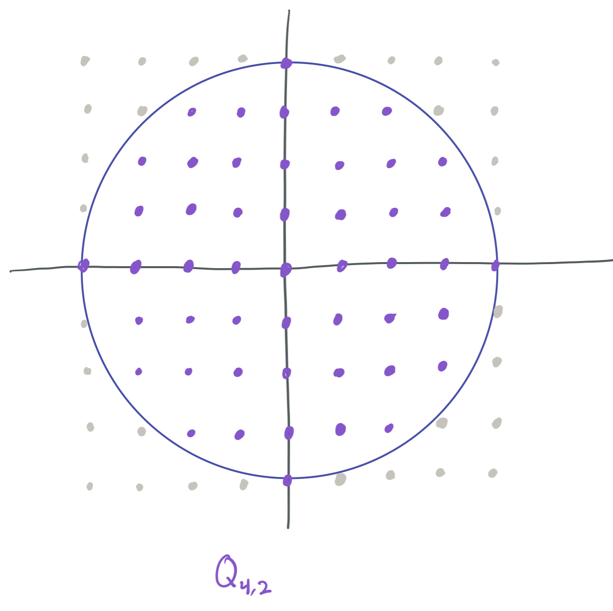
We can equivalently write the upper and lower bounds on the minimum width as \(Q_{2L/\epsilon, d}^{O(1)}\) and \(\Omega(Q_{L/18\epsilon, d})\) respectively. This combinatorial quantity turns out to be important for the proofs of both bounds.
A key building block for both proofs is an orthonormal basis. I define orthonormal bases in a different blog post and explain why they’re useful there. If you aren’t familiar, check that one out. We use the following family of sinusoidal functions as a basis for the \(L_2\) Hilbert space on \([-1, 1]^d\) throughout:
\[\mathcal{T} \approx \{T_K: x \mapsto \sqrt{2}\cos(\pi\langle K, x\rangle): K \in \mathbb{Z}^d\}.\]Note: This is an over-simplification of the family of functions to be easier to write down. Actually, half of the functions need to be sines instead of cosines. However, it’s a bit of a pain to formalize and you can see how it’s written up in the paper. I’m using the \(\approx\) symbol above because this is “morally” the same as the true family of functions, but a lot easier to write down.
This family of functions has several properties that are very useful for us:
-
The functions are orthonormal with respect to the Hilbert space for the \(L_2\) space over the uniform distribution on \([-1, 1]^d\). That is, for all \(K. K' \in \mathcal{T}\),
\[\langle T_K, T_{K'}\rangle = \mathbb{E}_{x}[T_K(x)T_{K'}(x)] = \begin{cases}1 & K = K' \\ 0 & \text{otherwise.} \\ \end{cases}\] - The functions span the Hilbert space \(L_2([-1,1]^d)\). Put together with the orthonormality, \(\mathcal{T}\) is an orthonormal basis for \(L_2([-1,1]^d)\).
- The Lipschitz constant of each of these functions is bounded. Specifically, the Lipschitz constant of \(T_K\) is at most \(\sqrt{2} \pi \|K\|_2\).
- The derivative of each function in \(\mathcal{T}\) is also a function that’s contained in \(\mathcal{T}\) (if you include the sines too).
- All elements of \(\mathcal{T}\) are ridge functions. That is, they can each be written as \(T_K(x) = \phi(\langle v, x \rangle)\) for some \(\phi:\mathbb{R}\to \mathbb{R}\).The function depends only on one direction in \(\mathbb{R}^d\) and is intrinsically one-dimension. This will be important for the upper bound proof.
- If we let \(\mathcal{T}_k = \{T_K \in \mathcal{T}: \|K\|_2 \leq k\}\), then \(\lvert\mathcal{T}_k\rvert = Q_{k,d}\).
Now, we’ll use this basis to discuss our proof of the upper bound.
A. Upper bound argument
The proof of the upper bound boils down to two steps. First, we show that the function \(f\) can be \(\frac{\epsilon}{2}\)-approximated by a low-frequency trigonometric polynomial (that is, a linear combination of sines and cosines in \(\mathcal{T}_k\) for some \(k = O(L^2 / \epsilon^2)\)). Then, we show that this trigonometric polynomial can be \(\frac{\epsilon}{2}\)-approximated in turn by an RBL ReLU network.
For the first step—which corresponds to Lemma 7 of the paper—we apply the fact that \(f\) can be written as a linear combination of sinusoidal basis elements. That is,
\[f(x) = \sum_{K \in \mathbb{Z}^d} \alpha_K T_K(x),\]where \(\alpha_K = \langle f, T_K\rangle\). This means that \(f\) is a combination of sinusoidal functions pointing in various directions of various frequencies. We show that for some \(k = O(L / \epsilon)\),
\[P(x) := \sum_{K \in \mathbb{Z}^d, \|K\|_2 \leq k} \alpha_K T_K(x)\]satisfies \(\|P - f\|_2 \leq \frac{\epsilon}{2}\). To do so, we show that all \(\alpha_K\) terms for \(\|K\|_2 > k\) are very close to zero in the proof of Lemma 8. The argument centers on the idea that if \(\alpha_K\) is large for large \(\|K\|_2\), then \(f\) is heavily influenced by a high-frequncy sinusoidal function, which means that \(\|\nabla f(x)\|\) must be large at some \(x\). However, \(\|\nabla f(x)\| \leq L\) by our smoothness assumption on \(f\), so too large values of \(\alpha_K\) contradict this.
For the second part, we show that \(P\) can be approximated by a linear combination of random ReLUs. To do so, we express \(P\) as a superposition of or expectation over random ReLUs. We show that there exists some parameter distribution \(\mathcal{D}\) (which depends on \(d, L, \epsilon\), but not on \(f\)) and some bounded function \(h(b, w)\) (which can depend on \(f\)) such that
\[P(x) = \mathbb{E}_{(b, w) \sim \mathcal{D}}[h(b, w)\sigma(\langle w, x\rangle + b)].\]However, it’s not immediately clear how one could find \(h\) and why one would know that \(h\) is bounded. To find \(h\), we take advantage of the fact that \(P\) is a linear combination of trigonometric sinusoidal ridge functions by showing that every \(T_K\) can be expressed as a superposition of ReLUs and combining those to get \(h\). The “ridge” part is key here; because each \(T_K\) is effectively one-dimensional, it’s possible to think of it being approximated by ReLUs, as visualized below:
Each function \(T_K\) can be closely approximated by a piecewise-linear ridge function, since it has bounded gradients and because it only depends on \(x\) through \(\langle K, x\rangle\). Therefore, \(T_K\) can also be closely approximated by a linear combination of ReLUs, because those can easily approximate piecewise linear ridge functions. This makes it possible to represent each \(T_K\) as a superposition of ReLUs, and hence \(P\) as well.
Now, \(f\) is closely approximated by \(P\), and \(P\) can be written as a bounded superpositition of ReLUs. We want to show that \(P\) can be approximated by a linear combination of a finite and bounded number of random ReLUs, not an infinite superposition of them. This last step requires sampling \(r\) sets of parameters \((b^{(i)}, w^{(i)}) \sim \mathcal{D}\) for \(i \in \{1, \dots, r\}\) and letting
\[g(x) := \frac{1}{r} \sum_{i=1}^r h(b^{(i)}, w^{(i)}) \sigma(\langle w^{(i)}, x\rangle + b^{(i)}).\]When \(r\) is large enough, \(g\) is a 2-layer RBL ReLU network that becomes a very close approximation to \(P\), which means it’s also a great approximation to \(f\). Such a sufficiently large \(r\) can be quantified with the help of standard concentration bounds for Hilbert spaces. This wraps up the upper bound.
B. Lower bound argument
For the lower bounds, we want to show that for any bottom-layer parameters \((b^{(i)}, w^{(i)})\) for \(1 \leq i \leq r\), there exists some \(L\)-Lipschitz function \(f\) such that for any choice of top-layer \(u^{(1)}, \dots, u^{(r)}\):
\[\sqrt{\mathbb{E}_x\left[\left(f(x) - \sum_{i=1}^r u^{(i)} \sigma(\langle w^{(i)}, x\rangle + b^{(i)})\right)^2\right]} \geq \epsilon.\]This resembles a simpler linear algebra problem: Fix any vectors \(v_1, \dots, v_r \in \mathbb{R}^N\). \(\mathbb{R}^N\) has a standard orthonormal basis \(e_1, \dots, e_N\). Under which circumstances is there some \(e_j\) that cannot be closely approximated by any linear combination of \(v_1, \dots, v_r\)?
It turns out that when \(N \gg r\) there can be no such approximation. This follows by a simple dimensionality argument. The span of \(v_1, \dots, v_r\) is a subspace of dimension at most \(r\). Since \(r \ll N\), it makes sense that an \(r\)-dimensional subspace cannot be close to every \(N\) orthonormal vector, since they lie in a much higher dimensional object and each is perpendicular to every other.
For instance, the above image illustrates the claim for \(N = 3\) and \(r = 2\). While the span of \(v_1\) and \(v_2\) is close to \(e_1\) and \(e_2\), the vector \(e_3\) is far from that plane, and hence is inapproximable by linear combinations of the two.
In our setting, we replace \(\mathbb{R}^N\) with the \(L_2\) Hilbert space over functions on \([-1, 1]^d\); \(v_1, \dots, v_r\) with \(x \mapsto \sigma(\langle w^{(1)}, x\rangle + b^{(1)}), \dots, x \mapsto \sigma(\langle w^{(r)}, x\rangle + b^{(r)})\); and \(\{e_1, \dots, e_N\}\) with \(\mathcal{T}_k\) for \(k = \Omega(L)\). As long as \(Q_{k,d} \gg r\), then there is some \(O(\|K \|_2)\)-Lipschitz function \(T_K\) that can’t be approximated by linear combinations of ReLU features. By the assumption on \(k\), \(T_K\) must be \(L\)-Lipschitz as well.
The dependence on \(\epsilon\) can be introduced by scaling \(T_K\) appropriately.
Parting thoughts
To reiterate, our results show the capabilities and limitations of 2-layer random bottom-layer ReLU networks. We show a careful interplay between the Lipschitzness of the function to approximate \(L\), the dimension \(d\), and the accuracy parameter \(\epsilon\). Our bounds rely heavily on orthonormal functions.
Our results have some key limitations.
- Our upper bounds would be more impressive if they used the \(L_\infty\) notion of approximation, rather than \(L_2\). (Conversely, our lower bounds would be less impressive if they used \(L_\infty\) instead.)
- The distribution over training parameters \(\mathcal{D}\) that we end up using for the upper bounds is contrived and depends on \(L, \epsilon, d\) (even if not on \(f\)).
- Our bounds only apply when samples are drawn uniformly from \([-1, 1]^d\). (We believe our general approach will also work for the Gaussian probability measure, which we discuss at a high level in the appendix of our paper.)
We hope that these limitations are addressed by future work.
Broadly, we think our paper fits into the literature on neural network approximation because it shows that the smoothness of a function is very relevant to its ability to be approximated by shallow neural networks.
- Our paper contributes to the question posed by SES19 (Are there any 1-Lipschitz functions that cannot be approximated efficiently by depth-2 but can by depth-3?) by showing that all 1-Lipschitz functions are approximable with respect to the \(L_2\) measure.
- In addition, our results build on those of a recent paper by Malach, Yehudai, Shalev-Shwartz, and Shamir (2021), that suggests that the only functions that can be efficiently learned via gradient descent by deep networks are those that can be efficiently approximated by a shallow network. They show that the inefficient approximation of a function by depth-3 neural networks implies inefficient learning by neural networks of any depth; our results strengthens this to “inefficient approximation of a function by depth-2 neural networks.”
Thank you so much for reading this blog post! I’d love to hear about any thoughts or questions you may have. And if you’d like to learn more, check out the paper or the talks!
Comments