[OPML#6] XH19: On the number of variables to use in principal component regression
[candidacy technical learning-theory over-parameterized least-squares This is the 6th of a sequence of blog posts that summarize papers about over-parameterized ML models.
Here’s another paper by my advisor Daniel Hsu and his former student Ji (Mark) Xu that discusses when overfitting works in linear regression. This one differs subtly from some of the previously discussed papers (like BHX19 [OPML#1] and BLLT19 [OPML#2]) in that it considers principal component regression (PCR) rather than least-squares regression.
Principal component regression
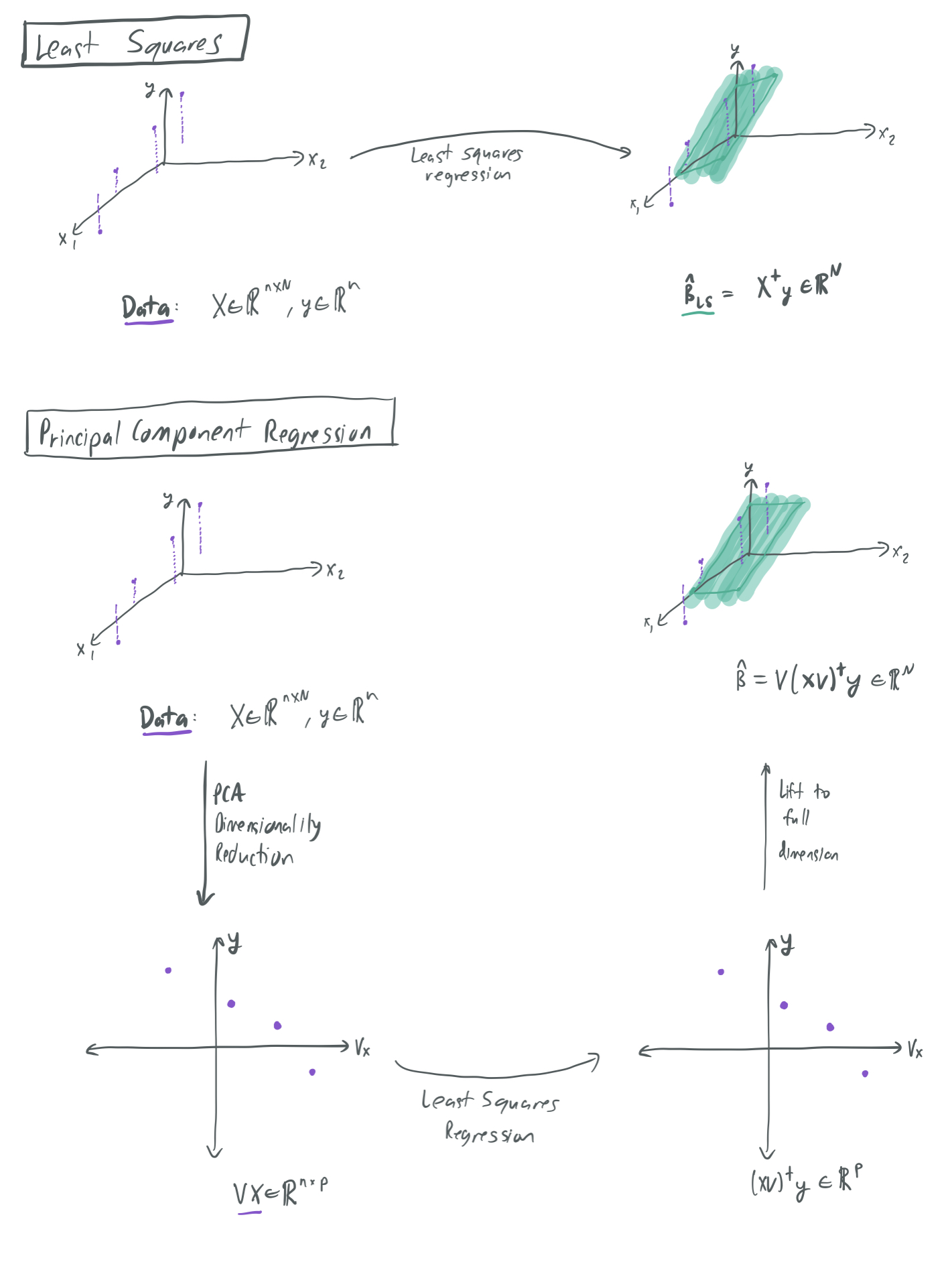
Suppose we have a collection of \(n\) samples \((x_i, y_i) \in \mathbb{R}^{N} \times \mathbb{R}\), which we collect in design matrix \(X \in \mathbb{R}^{n \times N}\) and label vector \(y \in \mathbb{R}^n\). The standard approach to least-squares regression (which has been given numerous times on this blog) is to choose the \(\hat{\beta}_\textrm{LS} \in \mathbb{R}^N\) that minimizes \(X \hat{\beta}_\textrm{LS} = y\), breaking ties by minimizing the \(\ell_2\) norm \(\|\hat{\beta}_{\textrm{LS}}\|_2\). This approach considers all dimensions of the inputs \(x_i\).
However, there might a situation where we know \(\Sigma\) a priori and only want to consider the directions in \(\mathbb{R}^N\) that the inputs meaningfully vary along. This is where principal component regression comes in. Instead of regressing on the training data itself, we regress on the \(p\) most significant dimensions of the data, as identified by principal component analysis (PCA). PCA is a linear dimensionality reduction method that obtains a lower-dimensional representation of \(X\) by approximating each sample as a linear combination of the \(p\) eigenvectors of \(X^T X\) with the largest corresponding eigenvalues. These \(p\) eigenvectors correspond to the directions in \(\mathbb{R}^N\) where the samples in \(X\) have highest variance. Moreover, projecting each of the \(n\) samples \(x_i\) onto the space spanned by these \(p\) eigenvectors provides the closest average \(\ell_2\)-approximation of each \(x_i\) as a linear combination of \(p\) fixed vectors in \(\mathbb{R}^N\).
Let \(\mathbb{E}[x_i] = 0\) and \(\Sigma = \mathbb{E}[x_i x_i^T]\) be the covariance matrix of \(x_i\). If we know \(\Sigma\) ahead of time, then we can simplify things by using only the eigenvectors of \(\Sigma\), rather than the empirical principal components taken from eigenvectors of \(X^T X\). If the \(p\) eigenvectors \(\Sigma\) with the largest eigenvalues are collected in \(V \in \mathbb{R}^{N \times p}\), then we can express the low-dimensional representation of the training samples as \(X V \in \mathbb{R}^{n \times p}\). By applying linear regression to these new low-dimensional samples and transforming the resulting parameter vector back to \(\mathbb{R}^N\), we get the parameter vector \(\hat{\beta} = V(X V)^{\dagger} y\), where \(\dagger\) denotes the pseudo-inverse. (On the other hand, the least-squares parameter vector is \(\hat{\beta}_\textrm{LS} = X^{\dagger} y\).)
The below image visualizes the differences between the least squares and PCR regression algorithms. It shows a toy example where samples \((x, y)\) (in purple) vary greatly in one direction and not much at all in another direction. PCR only considers the direction of maximum variance and rules the other out, while least squares considers all directions simultaneously. Therefore, the hypotheses represented by the green hyperplanes look subtly different for each case.
Note that this formulation of PCR concerns an idealized setting. Most regression tasks do not give the learner direct access to \(\Sigma\). However, it’s possible that \(\Sigma\) could be separately estimated with \(\hat{\Sigma}\) and then applied by PCA. They authors refer to this as “semi-supervised” because the \(\Sigma\) can be estimated with using only unlabeled samples, since none of the labels \(y\) are used in the approximation. Due to the high cost of obtaining labeled data, a sufficient dataset for kind of estimate may be significantly easier to obtain than a dataset for the general learning task.
Learning model and assumptions
They make several restrictive assumptions. The main purpose of this paper is to construct instances where favorable over-parameterization occurs for PCR, rather than exhaustively catalogue when it must occur.
They assume the samples \(x_i\) have independent Gaussian components and that labels \(y_i = \langle x_i, \beta\rangle\) have no noise. \(\Sigma\) is a diagonal matrix (which must be the case because of the independent components of each \(x_i\)) with entries \(\lambda_1 > \dots > \lambda_N > 0\). Therefore, PCR will only use the first \(p\) diagonal entries of \(\Sigma\) and the reduced-dimension version of each sample will merely be its first \(p\) entries.
One weird thing about this paper relative to others is that the true parameter vector \(\beta\) is chosen randomly. This means it’s an “average-case” bound. They justify this on the grounds that the ability to choose an arbitrary \(\beta\) could lead to all of the weight being put on the \(N-p\) components that will not be included the PCA’d version of \(X\). This would make it impossible to have non-trivial error bounds.
Over-parameterization and PCR
Now, we have three parameters to consider (\(N, p, n\)), rather than the two (\(p, n\)) typically considered in the previous works on over-parameterization. As before, they think of over-parameterization as the ratio \(\gamma = \frac{p}{n}\), but they must also contend with the ratios \(\alpha = \frac{p}{N}\) (the fraction of dimensions preserved by PCA) and \(\rho = \frac{n}{N}\) (the ratio of samples to original dimension).
Like HMRT19 [OPML#4], they consider what happens when \(N, p, n \to \infty\) and the ratios remain fixed. Like BLLT19, their results study how over-parameterization is affected as the eigenvalues of \(\Sigma\) change. In Section 2, they focus on eigenvalues \(\lambda_1, \dots, \lambda_N\) that decay predictably at a polynomial rate. Theorems 1 and 2/3 characterize what happens to the expected error in the under-parameterized (\(\gamma \leq 1\)) and over-parameterized (\(\gamma > 1\)) respectively.
- Theorem 1 shows that the shape of the “classical” regime error curve is preserved in the under-parameterized regime, since it shows that the error decreases as \(\alpha\) increases for fixed \(\rho\), up to a point when it decreases until \(\alpha = \rho\) (equivalently, \(p = n\)).
- Theorem 2 shows that the expected error in the interpolation regime \(p > n\) converges to some fixed risk quantity, which can be determined by evaluating an intergral and solving for some quantity.
- Theorem 3 shows that for any polynomial rate of decay of the eigenvalues, double-descent will occur and the best interpolating prediction rule will perform better than the best “classical” prediction rule. In the noisy setting, the best interpolating prediction rule will only outperform the best classical rule in the event that the rate of decay is no faster than \(\frac{1}{i}\).
To recap, the optimal performance for PCR is obtained in the over-parameterized regime (with \(p > n\)) if and only if eigenvalues \(\lambda_1, \dots, \lambda_N\) decay slowly; rapid decay leads to optimality in the classical regime. This echoes the results of BLLT19, which shows that too rapid a decay in eigenvalues causes poor performance in the over-paramterized regime (very-much-not-benign overfitting). However, BLLT19 also requires that the rate of decay not be too slow, which is a non-issue in this regime.
One of the nice things about this paper–which will be expanded on in the weeks to come–is that it separates the number of parameters \(p\) from the dimension \(N\). Talking about over-parameterization in linear regression is often awkward because the two quantities are coupled, and we are forced to ask whether favorable behavior in the over-parameterized regime is caused by the high dimension or the high parameter count. We’ll further examine models with separate dimensions and parameter counts when we study random feature models.
Comments