[OPML#7] BLN20 & BS21: Smoothness and robustness of neural net interpolators
[candidacy technical learning-theory over-parameterized This is the seventh of a sequence of blog posts that summarize papers about over-parameterized ML models, which I’m writing to prepare for my candidacy exam. Check out this post to get an overview of the topic and a list of what I’m reading.
This post discusses two papers by Sebastian Bubeck and his collaborators that are of interest to the study of over-parameterized neural networks. The first, “A law of robustness for two-layers neural networks” (BLN20) with Li and Nagaraj, gives a conjecture about the “robustness” of a two-layer neural network that interpolates all of the training data. The second, “A universal law of robustness via isoperimetry” (BS21) with Sellke, proves part of the conjecture and extends that part of the conjecture to deeper neural networks. The other part of the conjecture remains open for future work to tackle.
Both papers consider a setting where there are \(n\) training samples \((x_i, y_i) \in \mathbb{R}^d \times \{-1,1\}\) drawn from some distribution that are fit by a neural network with \(k\) neurons. For the two-layer case (which we’ll focus on in this writeup), they consider neural networks of the form
\[f(x) = \sum_{j=1}^k u_j \sigma(w_j^T x + b_j),\]where \(\sigma(t) = \max(0, t)\) is the ReLU activation function and \(w_j \in \mathbb{R}^d\) and \(b_j, u_j \in \mathbb{R}\) are the parameters. Roughly, they ask whether there exists a “smooth” neural network \(f\) such that \(f(x_i) \approx y_j\) for all \(j \in [n]\); this makes \(f\) an approximate interpolator.
How does this relate to the rest of this blog series? All of the other posts so far have been about cases where over-parameterized linear regression leads to favorable generalization performance. These generalization results occur due to the smoothness of the linear prediction rule. That is, if we have some prediction rule \(x \mapsto \beta^T x\) for \(x, \beta \in \mathbb{R}^d\) with \(d \gg n\), we might have good generalization if \(\|\beta\|_2\) is small, which is enabled when \(d\) is very large. The same observation holds up with neural networks (over-parameterized models leads to benign overfitting), but it’s harder to prove why it leads to a small generalization error. By understanding the smoothness of interpolating neural networks, it might make it easier to prove generalization bounds on the neural networks that perfectly fit the training data.
How do they measure smoothness? For linear regression, it’s natural to think of the smoothness of the prediction rule \(f_{\text{lin}}(x) = \beta^T x\) as \(\|\beta\|_2\), since that is the magnitude of the gradient \(\|\nabla f_{\text{lin}}(x)\|_2\) at every sample \(x\). For two-layer neural networks—which are non-linear functions—it’s natural instead to consider the maximum norm of the gradient of \(f\), which is represented by the Lipschitz constant of \(f\): the minimum \(L\) such that \(|f(x) - f(x')| \leq L \|x - x'\|_2\) for all \(x, x'\). (Lipschitzness also comes up frequently in my COLT paper about the approximation capabilities of shallow neural networks.)
What does it have to do with robustness? Typically, robustness is discussed in the context of adversarial examples. If you’ve hung around the ML community, you’ve probably seen this issue featured in images like this:
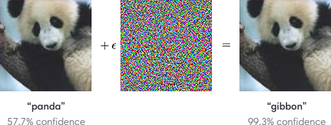
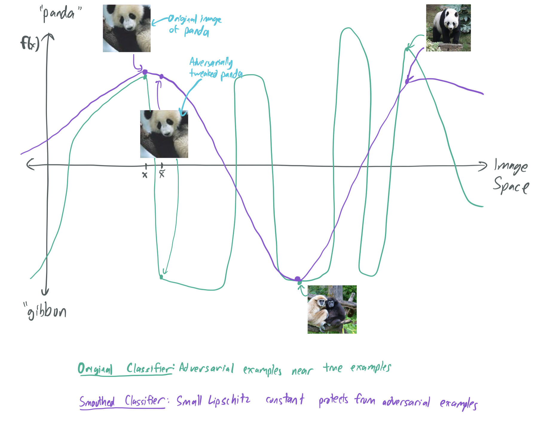
Here, an image of a panda is provided that a trained image classification neural network clearly identifies as such. However, a small amount of noise can be added to the image that leads to the network being tricked into thinking that it’s a gibbon instead. Put roughly, it means that the network outputs \(f(x) = \text{"panda"}\) and \(f(x + \epsilon \tilde{x}) = \text{"gibbon"}\) for some \(x\) and \(\tilde{x}\), which means that the output of \(f\) changes greatly near \(x\). By mandating that \(f\) have a small Lipschitz constant, these kinds of fluctuations are impossible. This makes the network \(f\) robust. Thus, enforcing smoothness conditions is a way to ensure that a predictor is robust to these kinds of adversarial examples.
As a result, Bubeck and his collaborators want to characterize the availability of interpolating networks \(f\) that are also robust, with the hopes of understanding how over-parameterization can be used to avoid having adversarial examples.
One important caveat: Unlike the previous papers discussed in this series, this one focuses only on approximation and not optimization. It asks whether there exists an interpolating prediction rule that is smooth, but it does not ask whether this rule can be easily obtained from stochastic gradient descent.
For the rest of the post, I’ll discuss the conjecture made by BLN20, share the support for the conjecture that was provided by BLN20 and BS21, and discuss what remains to be studied in this space.
The conjecture
For simplicity, BLN20 considers only samples drawn uniformly from the unit sphere: \(x \in \mathbb{S}^{d-1}= \{x \in \mathbb{R}^d: \|x\|_2=1\}\) with iid labels \(y_i \sim \text{Unif}(\{-1,1\})\). The conjecture of BLN20, which combines their Conjectures 1 and 2 is as follows:
Consider some \(k \in [\frac{cn}{d}, Cn]\) for constants \(c\) and \(C\). With high probability over \(n\) random samples from some distribution, there exists a 2-layer neural network \(f\) of width \(k\) that perfectly fits the data such that \(f\) is \(O(\sqrt{n/k})\)-Lipschitz. Furthermore, any neural network that fits the data must be \(\Omega(\sqrt{n/k})\)-Lipschitz with high probability.
If true, the conjecture suggests there can only be an \(O(1)\)-Lipschitz interpolating neural network \(f\) if the model is highly over-parameterized, or \(k = \Omega(n)\). Note that \(k\) is the number of neurons, and not the number of parameters. In the case of a 2-layer neural network, the number of parameters is \(p = kd\), so there must be at least \(p = \Omega(nd)\) parameters for the interpolating network to be smooth.
The conditions with constants \(c\) and \(C\) are necessary for the question to be well-posed.
- Without the \(k \leq Cn\) constraint, there theorem would imply the existence of neural networks that fit the data and are \(o(1)\)-Lipschitz. However, this is not possible unless all training samples are have the same label \(y_i\); otherwise, there are at least two different samples \(x_i\) and \(x_j\) that are at most distance 2 apart (since both lie on \(\mathbb{S}^{d-1}\)) and have opposite labels. This implies that any function fitting both samples must be at least 1-Lipschitz.
- Without the \(k \geq \frac{cn}{d}\) constant, there is unlikely to exist any neural network with \(k\) neurons that can fit the \(n\) samples. Since the number of parameters \(p\) is roughly \(kd\), letting \(k \ll \frac{n}{d}\) would ensure that \(p \ll n\) and there are fewer parameters than samples. Intuitively, it’s difficult to fit a large number of points with random labels when there are fewer parameters than samples. This suggests that the model must be over-parameterized for interpolation to even occur in the first place, let alone be smooth.
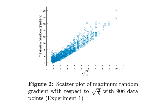
BLN20 shows that the conjecture holds up empirically on toy data. For many values of \(n\) and \(k\), they train several neural networks to fit the \(n\) samples with 2-layer neural networks of width \(k\) and randomly sample gradients to find the one with the largest magnitude. When plotted, they note a nice linear relationship between the norms of the largest random gradient and \(\sqrt{n/k}\). Of course, the maximum random gradient is not the same as the Lipschitz constant, since it’s impossible to check the gradient for all values of \(x\) simultaneously, but this suggests that it’s likely that the conjecture is correct.
Partial upper bounds from BLN20
The BLN20 papers focuses on presenting the conjecture and giving a series of partial results that suggest it may be true. In this section, we give a brief summary of each of the partial solutions.
The following are all partial solutions to the upper bound. That is, they show weaker versions of the claim that there exists neural network \(f\) with Lipschitz constant \(O(\sqrt{n/ k})\) by showing either larger bounds on the Lipschitz constant or more restrictive parameter regimes.
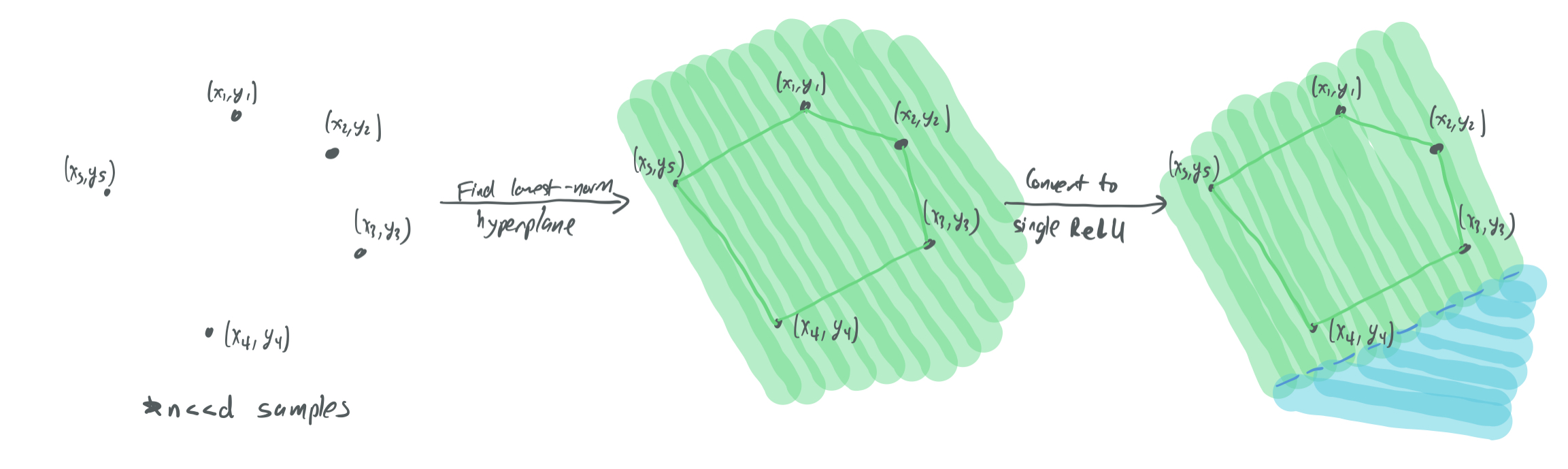
- The high-dimensional case (3.1). If \(d \gg n\), then a ReLU network with a single neuron \(k = 1\) can be used to perfectly fit the data.
This is because a single \(d\)-dimensional hyperplane will be able to fit the \(n\) samples, so one can just choose the hyperplane with the lowest magnitude that fits the data and use a ReLU that corresponds to that hyperplane. By similar analysis to that of linear regression, the Lipschitz constant of this network will be \(O(\sqrt{n})\) with high probability, which is the same as \(O(\sqrt{n/ k})\). This can’t be improved without using more neurons.
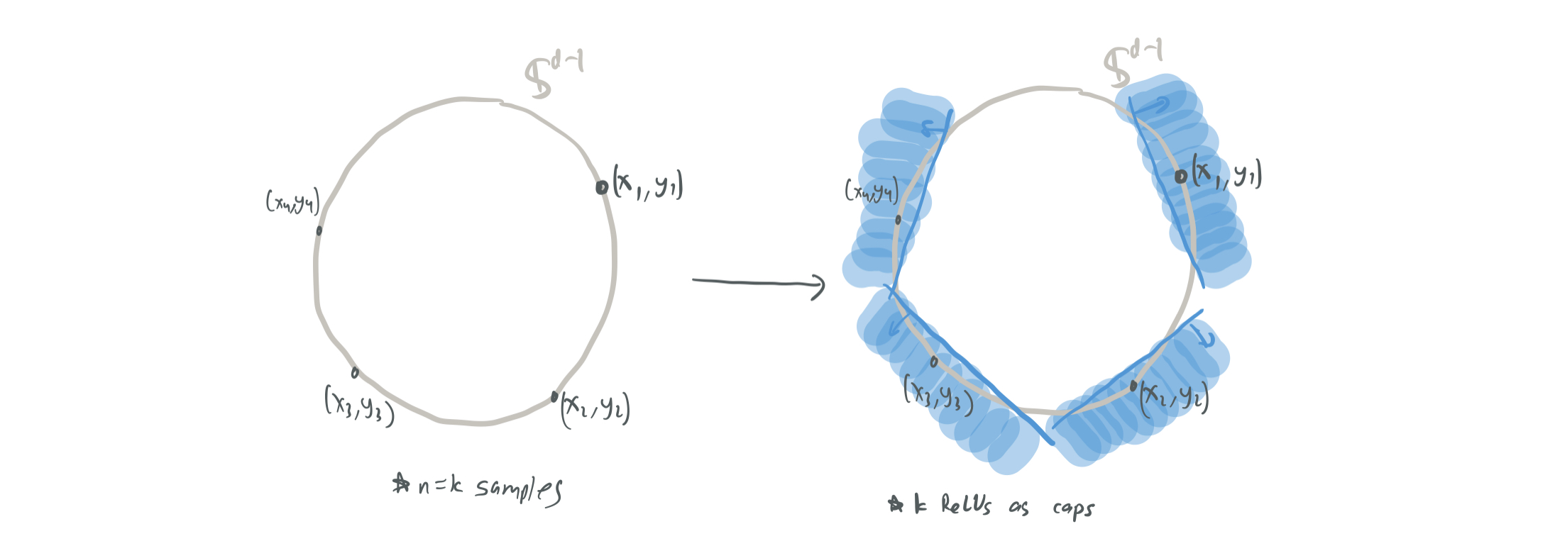
- The wide (“optimal size”) regime: \(k = n\) (3.2). With high probability, an \(10\)-Lipschitz network \(f\) can be provided by using a ReLU for every sample. Each ReLU is treated as a “cap” that gives a sample the correct label. With high probability, the points will be sufficiently spread apart in \(\mathbb{S}^{d-1}\) to ensure that none of the the caps overlap. This makes the norm of the gradient never more than \(10\), if each cap is offset by \(\frac{1}{10}\).
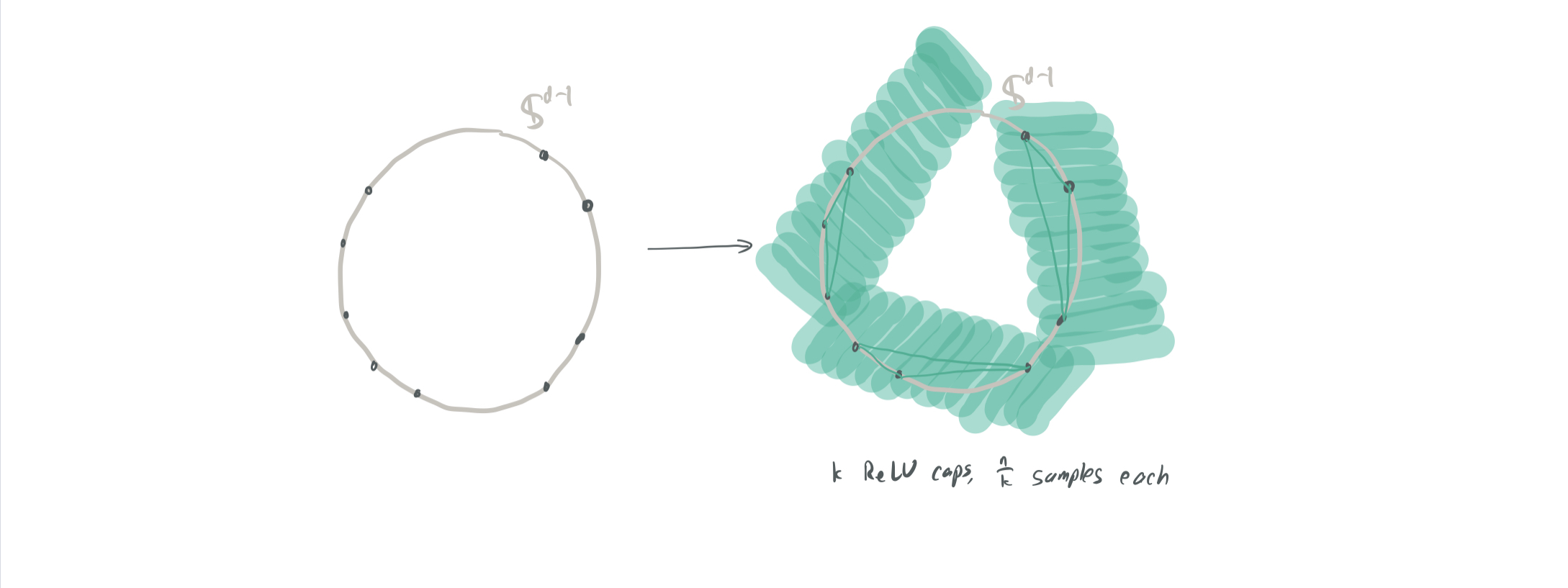
- The compromise case (3.3). The two previous approaches can be combined for a broader choice of \(k\) and \(n\) by instead having each ReLU perfectly fit \(m := n/k \leq d\) samples in a cap. However, since these are bigger and more complex caps then before, we need to be more concerned about the caps overlapping. They show that \(O(m \log d)\) caps will overlap at any given point, which means that the Lipschitz constant will be \(O(n\log (d) / k)\). Even disregarding the logarithmic factor, this is still much weaker than the \(O(\sqrt{d/k})\) factor that the conjecture desires.
- The very low-dimensional case with a weird architecture (3.4).
They prove the existence of a neural network that fits \(n\) samples and has Lipschitz constant \(O(\sqrt{n / k})\) with high probability. To do so, however, they need several major caveats:
- The dimension \(d\) is very small; for some constant even integer \(q\), \(k = C_q d^{q-1}\) and \(n \approx \frac{d^q}{100 q \log d}\), where \(C_q\) depends on \(q\). Note that the number of neurons \(k\) can be much bigger than the number of samples \(n\) when \(d\) is very small and \(q\) is large.
- \(f\) approximately interpolates the samples. That is, \(\lvert f(x_i) - y_i\rvert \leq 0.1 C_q\) for all \(i \in [n]\). (Note that 0.1 can be replaced by \(\epsilon\) and the result can be generalized.)
- The neural network uses the activations \(t \mapsto t^q\) and not the ReLU function.
This can be thought of as a tensor interpolation problem. Specifically, for \(q = 2\), they perform regression on the space \(x^{\otimes 2} = (x_1^2, x_1x_2, \dots, x_1 x_d,\dots x_2x_1, x_2^2, \dots, x_d^2)\) using the quadratic activation function. This approach gives the kind of bound they’re looking for, but is a strange enough case that it’s unclear how to extend this to networks with (1) high input dimensions, (2) perfect interpolation, and (3) ReLU activations.
The paper also gives a few constrained versions of the lower bound on the Lipschitz constant for any interpolating function. However, we omit them here because the second paper—BS21—has much better lower bounds.
Lower bound from BS21
The follow-up paper proves a mostly-tight lower bound, which effectively resolves half of the conjecture. The results require isoperimetry to hold, which is true of a random variable \(x \in \mathbb{R}^d\) if \(f(x)\) has subgaussian tails for every Lipschitz function \(f\). This holds for well-known distribution such as (1) multivariate Gaussian distributions, (2) the uniform distribution on \(\mathbb{S}^{d-1}\), (3) and the uniform distribution on the hypercube \(\{-1, 1\}^d\).
By combining their Lemma 3.1 and Theorem 3, the following statement is true about 2-layer neural networks:
Let \(\mathcal{F}\) be a family of 2-layer neural networks of width \(k\) with parameters in \([-W, W]\). Suppose each sample \((x_i, y_i)\) is drawn from isoperimetric distribution for all \(i \in [n]\) with \(\mathbb{E}[\mathrm{Var}[y \mid x]] > 0.1\) and such that \(\| x_i \|_2 \leq R\) almost surely. Then, with high probability, any neural network \(f \in \mathcal{F}\) that perfectly fits all \(n\) training samples will have a Lipschitz constant of
\[\Omega\left(\sqrt{\frac{n}{k \log (W R nk)}}\right).\]This is close to the conjecture up to logarithmic factors! In addition, this result is more general in the paper:
- Instead of considering only depth-2 neural networks, they consider all parametric models that change by bounded amounts as their parameter vectors change.
- Within their study of neural networks, their analysis also addresses networks that share parameters.
- A parameter \(\epsilon\) allows them to conclude that all networks that nearly interpolate must have high Lipschitz constant, not just those that perfectly fit the data.
They also account for the fact that the bounds on parameter weights with \(W\) are necessary. Through their Theorem 4, they show the existence of a neural network with a small Lipschitz constant that approximates nearly all of the samples with only a single parameter. Thus, without these kinds of assumptions, the conjecture is rendered uninformative.
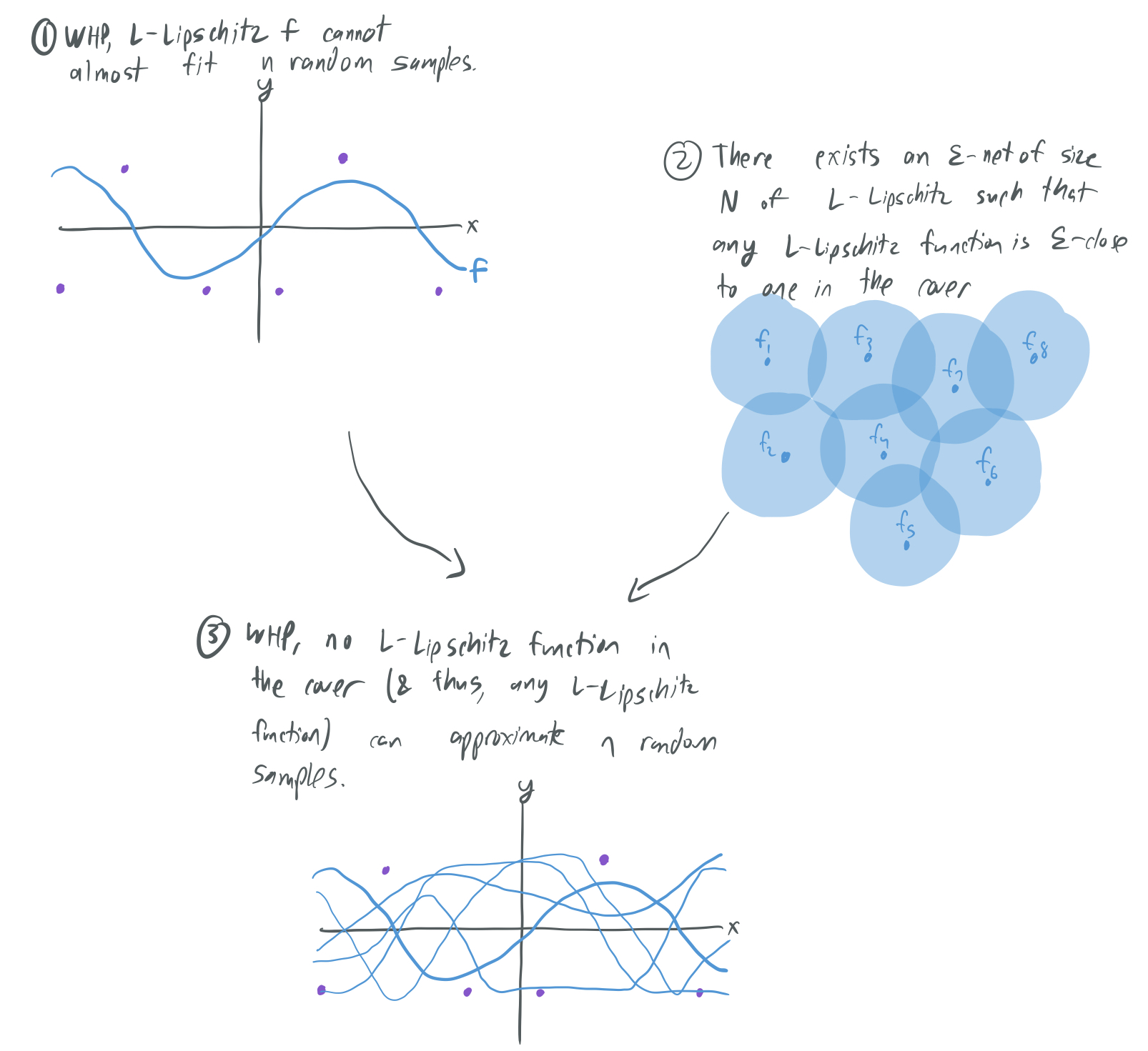
The proof works by considering some fixed \(L\)-Lipschitz function \(f\) and asking how likely it is that \(n\) random samples are almost perfectly fit by \(f\). By isoperimetry, this can be shown to happen with very low probability. Then, by making use of an \(\epsilon\)-net argument, one can show that no \(L\)-Lipschitz function \(f\) can perfectly fit the samples.
While I breezed over the argument here, it’s a relatively simple one that can be followed by most people with some background in concentration inequalities.
Further questions
While the second paper resolves half of the open question from the first paper, the other half (the existence of a smooth interpolating neural network) remains open.
There are also a few caveats from the second paper that remain to be resolved. For one, it may be possible to loosen the restriction that there be non-zero label noise (i.e. \(\mathbb{E}[\mathrm{Var}[y \mid x]] > 0.1\)). In addition, the fact that \(\|x_i\|\) must always be bounded is a weakness, since it rules out Gaussian inputs; perhaps this could be improved.
Thanks for tuning in to this week’s blog post! See you next time!
Comments