[OPML#9] CL20: Finite-sample analysis of interpolating linear classifiers in the overparameterized regime
[candidacy technical learning-theory over-parameterized This is the ninth of a sequence of blog posts that summarize papers about over-parameterized ML models, which I’m writing to prepare for my candidacy exam. Check out this post to get an overview of the topic and a list of what I’m reading.
Like last week’s post, we’ll step away from linear regression and discuss how over-parameterized classification models can achieve good generalization performance. Unlike last week’s post, we focus on maximum-margin classifiers (or support vector machines) that interpolate the data in high-dimensional settings. The paper is called “Finite-sample Analysis of Interpolating Linear Classifiers in the Overparameterized Regime” and was written by Nilidri Chatterji and Philip Long.
Maximum-margin classifier
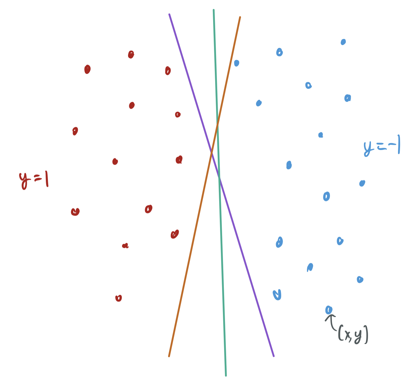
Suppose we have some linearly separable training data. There are many different strategies of choosing a linear separator for those data, and it’s unclear off the bat which ones will generalize best to novel samples. To sketch the issue, the below visualization shows how two linearly separable classes have many valid hypotheses that interpolate the training data and have zero training error.
The maximum-margin classifier chooses the separating hyperplane that, well, maximizes the margins between the separator and the two classes. In the below visualization, the yellow separator is the hyperplane orthogonal to the vector \(w\) that most decisively classifies every positive and negative sample correctly. That is, none of the sample are close to the separator, and \(w\) is chosen to have the largest margin, or gap between the data and the separator. The space between the solid separator and the two dashed lines is the margin, a sort of demilitarized zone between the two classes of samples.
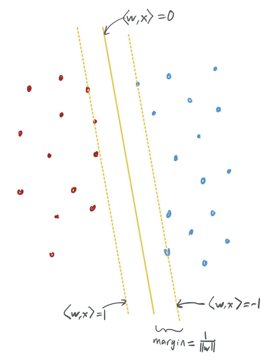
In order to quantify the margin, we require that \(w\) is chosen to ensure that \(\langle w, x_i\rangle \geq y_i\) for \(y_i \in \{-1,1\}\). The width of the margin can be computed to be at least \(\frac1{\|w\|}\) if we enforce this requirement. Therefore, maximum-margin classifier is
\[\mathop{\mathrm{arg\ min}}_{w \in \mathbb{R}^p} \|w\|, \text{ such that } \langle w, x_i\rangle \geq y_i, \ \forall i \in [n],\]where \((x_1, y_1), \dots, (x_n, y_n) \in \mathbb{R}^p \times \{-1, 1\}\) are the training samples.
Last week’s blog post discussed in detail why maximum-margin classifiers can lead to good generalization. Primarily, having large margins means that the classifier is robust and will categorize correctly samples that are drawn near any of the training samples. This is great, and provided a ton of insight into why overfitting is not always a bad thing. However, those results were limited in their applicability:
- They only apply to voting-based classifiers with margins, and this maximum-margin classifier does not directly aggregate together multiple weak classifiers. (One could think of a linear combination of features as being a combination of other classifiers, but those are not explicitly spelled out in the maximum-margin classifier.)
- Their bounds only apply to perfectly clean training data; if an \(\eta\)-fraction of the samples have incorrect labels, then their bounds fall apart.
This paper suggests that these kinds of bounds are possible for the maximum margin classifier when the dimension is much larger than the number of samples.
Aside: Their formulation of the maximum-margin classifier is identical to that of the support vector machine (SVM). The samples that lie on the margin (in our case, two red samples and two blue samples on the dotted lines) are support vectors, which the separator can be written in terms of. Classical capacity-based generalization approaches for SVMs relies on having few support vectors, but some recent works have shown that generalization bounds can be proved in a setting with many support vectors. One of my papers, which will appear at NeurIPS 2021 (and which I’ll discuss in a forthcoming blog post) proves when support vector proliferation , a phenomena where every samples is a support vector, occurs.
Data model
Like the linear regression papers we’ve discussed, this paper exhibits the phenomenon of benign overfitting under strict distributional assumptions. We present a simplified version of their data model below.
- A label \(\tilde{y} \in \{-1,1\}\) is chosen by a coin flip. With probability \(\eta\) (which can be no larger than some constant less than 1), the label is corrupted and \(y = - \tilde{y}\). Otherwise, \(y = \tilde{y}\).
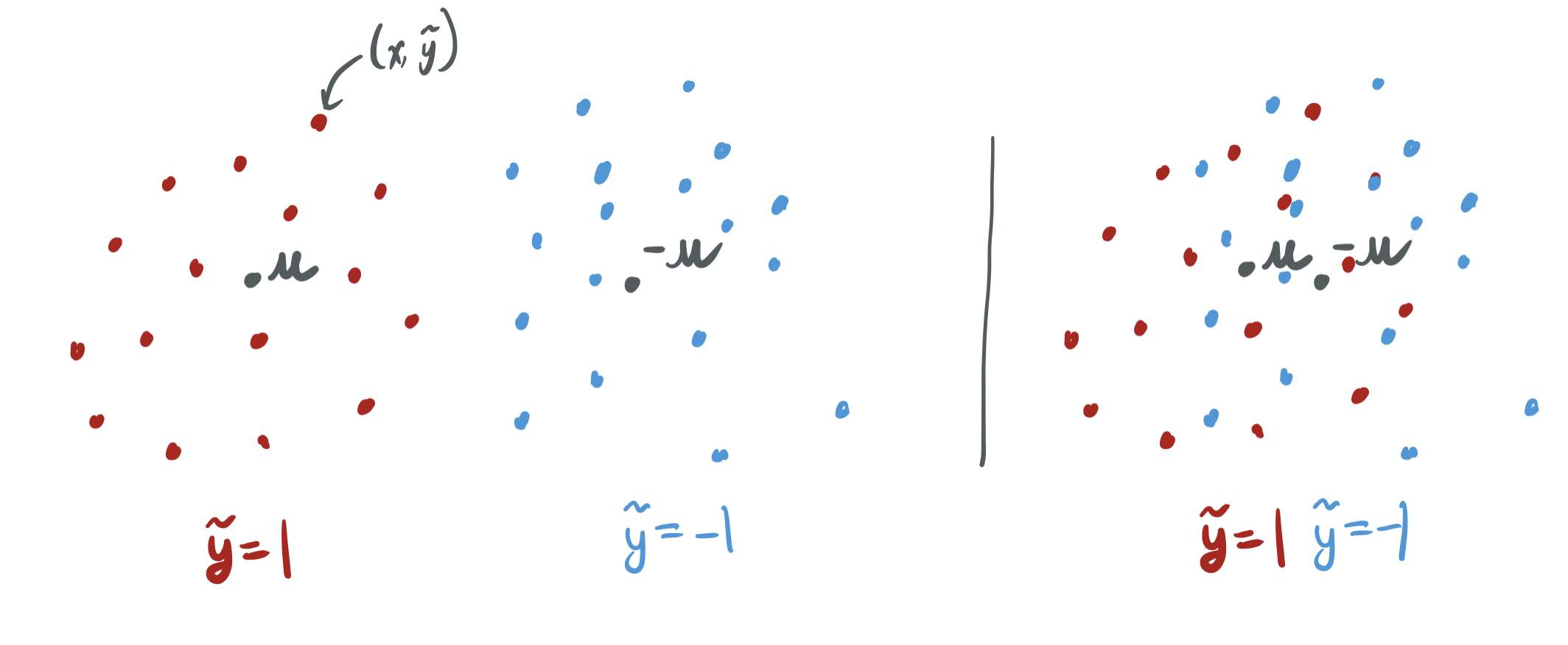
- For some mean vector \(\mu \in \mathbb{R}^p\) and some \(q\) drawn from a \(p\)-dimensional subgaussian distribution with a lower-bound on expected norm, the input \(x\) is chosen to be \(q + \tilde{y} \mu\).
That is, the inputs belong to one of two regions: either clustered around \(\mu\) if \(\tilde{y} = 1\) and \(-\mu\) if \(\tilde{y} = -1\). Intuitively, this means the learning problem is much easier if \(\mu\) is large, because the clusters will be more sharply separated.
The data model is limited by the fact that they assume this kind of two-cluster structure. However, it’s intended as a proof of concept of sorts, and the setup allows one to explore how changing the number of samples \(n\), the dimension \(d\), and the distinctiveness of classes \(\|\mu\|^2\) shapes which bounds are possible.
They give several examples of this data model, and I’ll recount their Example 3, which they call the Boolean noisy rare-weak model. They sample \(y\) and \(\tilde{y}\) as above. \(x\) is drawn from a distribution over \(\{-1,1\}^p\), where \(x_1, \dots, x_s\) independently equal \(\tilde{y}\) with probabililty \(\frac12 + \gamma\) and \(-\tilde{y}\) otherwise, for some \(s \leq p\) and \(\gamma \in (0, \frac12)\). \(x_{s+1}, \dots, x_p\) are the results of independent fair coin tosses.
Main result
Their main result is a generalization bound for this two-cluster data model. The result relies on several assumptions about \(n\), \(d\), and \(\mu\).
Theorem 4: Suppose (1) \(n\) is at least some constant, (2) \(p = \Omega(\max(\|\mu\|^2n, n^2 \log n))\), (3) \(\|\mu\|^2 = \Omega(\log n)\), and (4) \(p = O(\|\mu\|^4 / \log(1/\epsilon))\) for some \(\epsilon >0\). Then,
\[\mathrm{Pr}_{x,y}[\mathrm{sign}(\langle w, x\rangle \neq y)] \leq \eta + \epsilon,\]where \(w\) solves the max-margin optimization problem.
The main inequality is a bound on the generalization error of the classifier \(w\) because it deals with new samples, rather than the ones used to train the classifier. The \(\eta\) term in the error is unavoidable, because any sample will be corrputed with probability \(\eta\). The \(\epsilon\) term is the more interesting one, which governs the excess error.
The requirement that \(p = \Omega(n^2 \log n)\) means the model must be in a very high-dimensional regime. Recall that papers like HMRT19 consider a regime where \(p = \Theta(n)\); here, this paper only says anything about generalization when \(p\) is much larger than \(n\). We also require pretty specific conditions about \(\mu\).
To make life easier, let \(\mu = (q, 0, \dots, 0) \in \mathbb{R}^p\). The excess error can only be small then if \(q \gg p^{1/4}\). Since it must also be the case that \(q \ll \sqrt{p/ n}\), this gives a relatively narrow interval that \(p\) can belong to.
They formulate the theorem specifically for the example we consider as well.
Corollary 6: For the Boolean noisy rare-weak model, suppose (1) \(n\) is at least some constant, (2) \(p = \Omega(\max(\gamma^2 s n, n^2 \log n))\), (3) \(\gamma^2 s = \Omega(\log n)\), and (4) \(p = O(\gamma^4 s^2 / \log(1/\epsilon))\) for some \(\epsilon >0\). Then,
\[\mathrm{Pr}_{x,y}[\mathrm{sign}(\langle w, x\rangle \neq y)] \leq \eta + \epsilon,\]where \(w\) solves the max-margin optimization problem.
This means that if \(\gamma\) is some constant like \(0.25\), it must be true that \(s \gg \sqrt{p}\) and \(s \ll p/n\). Therefore, only a small fraction of the dimensions of \(x\) can be indicative of the label \(y\), and most of the input is just noise. Or, if \(s = p\) and every feature is significant, then \(\gamma\) must satisfy \(\gamma \ll 1/\sqrt{n}\) and \(\gamma \gg 1 / p^{1/4}\), which means that each feature will only have a minute amount of signal. This closely resembles the kinds of settings that we showed have good generalization for linear regression in BLLT19 long ago.
Proof overview
The proof relies on a proof by SHNGS18 that using gradient descent to optimize logistic regression for separable data gives a separating hyperplane that maximizes margins. That is, gradient descent with a logistic loss function has an implicit bias that leads to the same solution as to that of an SVM.
In Lemma 9, they use a simple concentration bound to show that the generalization error is small if \(\langle w, \mu\rangle\) is small, where \(\mu\) is the mean vector and \(w\) is the learned classifier. They relate this to the classifiers obtained in each step of gradient descent \(v^{(t)}\) and bound \(\langle v^{(t)}, \mu\rangle\) by expanding the gradient step to write \(v^{(t)}\) in terms of all previous risks. Taking a limit of \(t \to \infty\) relates this to the maximum-margin classifier.
Lemma 10 lower-bounds the target inner product. A key component of the proof of that is Lemma 14, which shows that the loss caused by any one sample cannot be much more than that of any other sample with high probability. This is important because it means that the noisy samples (with flipped \(\mu\)) cannot have outsize impact on the result, and that the analysis is robust to those errors.
Wrap up
This paper was neat, since it showed something similar to what was uncovered about minimum-norm linear regression by a variety of papers previously surveyed. It’s neat to also see this as a strengthening of the margin work discussed last week under boosting, since these results work for samples with noisy labels and for non-voting margin-based classifiers.
However, they’re limited by degree of over-parameterization/the size of the dimension needed; \(p = \Omega(n^2 \log n)\) is a pretty steep requirement, especially since results like my OLS=SVM paper suggest that minimum-norm regression (with samples drawn with labels in \(\{-1,1\}\)) and maximum-margin classifiers coincide when \(p = \Omega(n \log n)\). They specifically identify the improvement on the dependence of \(p\) as motivation for future work, and I hope to see that tackled at some point.
Thanks for reading this week’s entry! The actual exam is coming up on November 16th, and you should expect at least two more posts about papers before then!
Comments