[OPML#8] FS97 & BFLS98: Benign overfitting in boosting
[candidacy technical learning-theory over-parameterized This is the eighth of a sequence of blog posts that summarize papers about over-parameterized ML models, which I’m writing to prepare for my candidacy exam. Check out this post to get an overview of the topic and a list of what I’m reading.
In other news, there’s a cool Quanta article that touches on over-parameterization and the analogy between neural networks & kernel machines that just came out. Give it a read!
When conducting research on the theoretical study of neural networks, it’s common to joke that one’s work was “scooped” by a paper in the 1990s. There’s a lot of classic ML theory work that was published well before the deep learning boom of the last decade. As a result, it’s common for researchers to ignore it and unknowingly repackage old ideas as novel.
This week, I finally escape my pattern of discussing papers from the ’10s and ’20s by presenting a pair of seminal papers from the late ’90s: FS97 and BFLS98. Both of these papers cover boosting, a learning algorithm that aggregates many weak learners (heuristics that perform just better than chance) into a much better prediction rule.
- FS97 introduces the AdaBoost algorithm, proves that it can combine weak learners to perfectly fit a training dataset, and gives generalization bounds based on VC-dimension. The authors note that empirically, the algorithm performs much better than these capacity-based bounds and exhibits some form of benign overfitting (which has been extensively discussed in posts like [OPML#1], [OPML#2], [OPML#3], and [OPML#6]).
- BFLS98 addresses that mystery and resolves it by giving a different type of generalization bound, a margin-based bound, which explains why the generalization performance of AdaBoost continues to improve after it correctly classifies the training data.
These papers fit into the series because they exhibit a very similar phenomenon to the one we frequently encounter with over-parameterized linear regression and in deep neural networks: A learning algorithm is trained to zero training error and has small generalization error, despite capacity-based generalization bounds suggesting that this should not occur. Moreover, the generalization error continues to decrease as the model becomes “more over-parameterized” and continues to train beyond zero training error. These papers highlight the significance of margin bounds, which have been studied in papers like these in the context of neural network generalization.
We’ll jump in by explaining boosting, before discussing capacity-based and margin-based generalization bounds and the connection to benign overfitting.
Boosting
We motivate and discuss the boosting algorithm presented in FS97.
Population, training, and generalization errors
To motivate the problem, consider a setting where the goal is to learn a classifier from training data. That is, you (the learner) have \(m\) samples \(S = \{(x_1, y_1), \dots, (x_m, y_m)\} \subset X \times \{-1,1\}\) drawn independently from some distribution \(\mathcal{D}\). The goal is to learn some hypothesis \(h: X \to \{-1,1\}\) with low population error, that is
\[\text{err}_{\mathcal{D}}(h) = \text{Pr}_{(x, y) \sim \mathcal{D}}[h(x) \neq y].\]To do so, we follow the strategy of empirical risk minimization, that is choosing the \(h\) that minimizes training error:
\[\text{err}_S(h) = \sum_{i=1}^m \mathbb{1}\{h(x_i) \neq y_i\}.\]Often, the goal is to obtain a PAC learning (Probably Approximately Correct learning) guarantee, which entails showing that there exists some learning algorithm that gives a hypothesis \(h\) with probability \(1 - \delta\) such that \(\text{err}_{\mathcal{D}}(h) \leq \epsilon\) in time \(O(\frac{1}{\epsilon}, \frac1\delta)\) for any small \(\epsilon, \delta > 0\).
We can decompose the population error into two terms and analyze when algorithms succeed and fail based on the two:
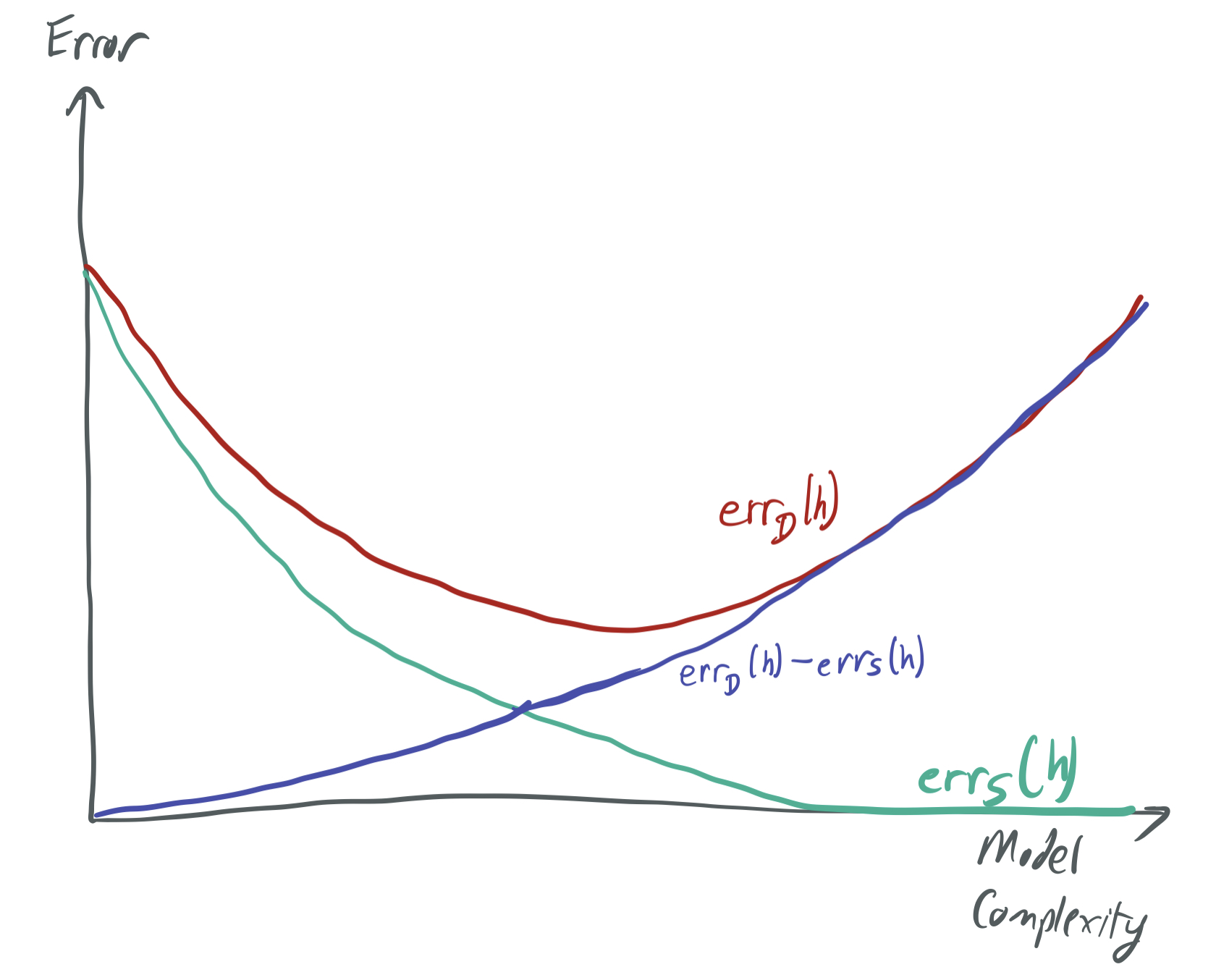
\[\text{err}_{\mathcal{D}}(h) = \underbrace{\text{err}_{\mathcal{D}}(h)-\text{err}_S(h)}_{\text{generalization error}} + \underbrace{\text{err}_S(h).}_{\text{training error}}\]This framing implies two very different types of failure modes.
- If the training error is large when \(h\) is an empirical risk minimizing hypothesis, then there is a problem with expressivity. In other words, there is no hypothesis that closely fits the training data, which means that there is very likely no hypothesis will succeed on random samples drawn from \(\mathcal{D}\).
- If the generalization error is large, then the sample \(S\) is not representative of the distribution \(\mathcal{D}\). Overfitting refers to the issue where the training error is small and the generalization error is large; the hypothesis does a good job memorizing the training data, but it learns little of the actual underlying learning rule because there aren’t enough samples. This typically occurs when \(h\) comes from a family of hypotheses that are too complex.
We can visualize these trade-offs with respect to the model complexity below, as they’re understood by traditional capacity-based ML theory. (There’s a very similar image in the introductory post of this blog series.)
While these blog posts focus on problematizing this picture by exhibiting cases where there is both overfitting and low generalization error, we introduce boosting in the context of solving the opposite problem: What do you do when the model complexity is too low, and no hypotheses do a good job of even fitting the training data?
Limitations of linear classifiers
Consider the following picture:
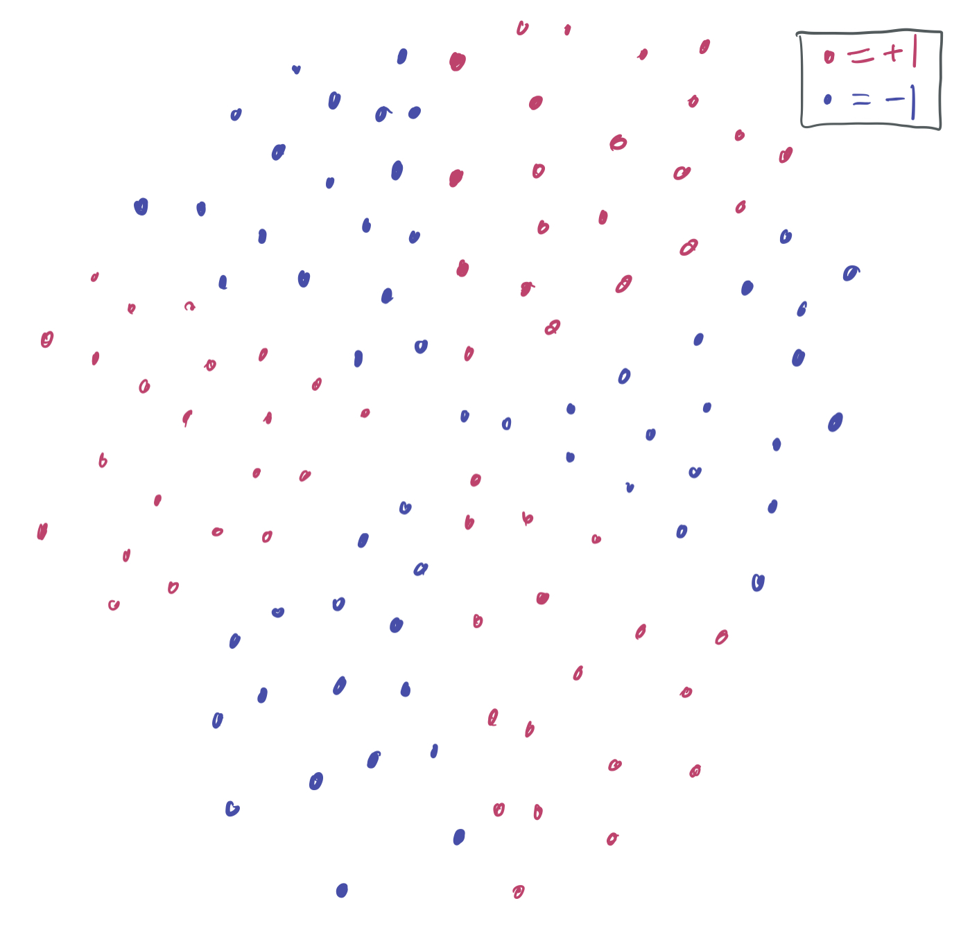
Suppose our goal is to find the best linear classifier that separates the red data (+1) from the blue data (-1) and (ideally) will also separate new red data from new blue data. However, there’s an immediate problem: no linear classifier can be drawn on the training data without a training error better than \(\frac13\). For instance, the following separator (which labels everything with \(\langle w, x\rangle > 0\) red and everything else blue) for some vector \(w \in \mathbb{R}^2\) performs poorly on the upper “slice” of red points and the lower slice of blue points.
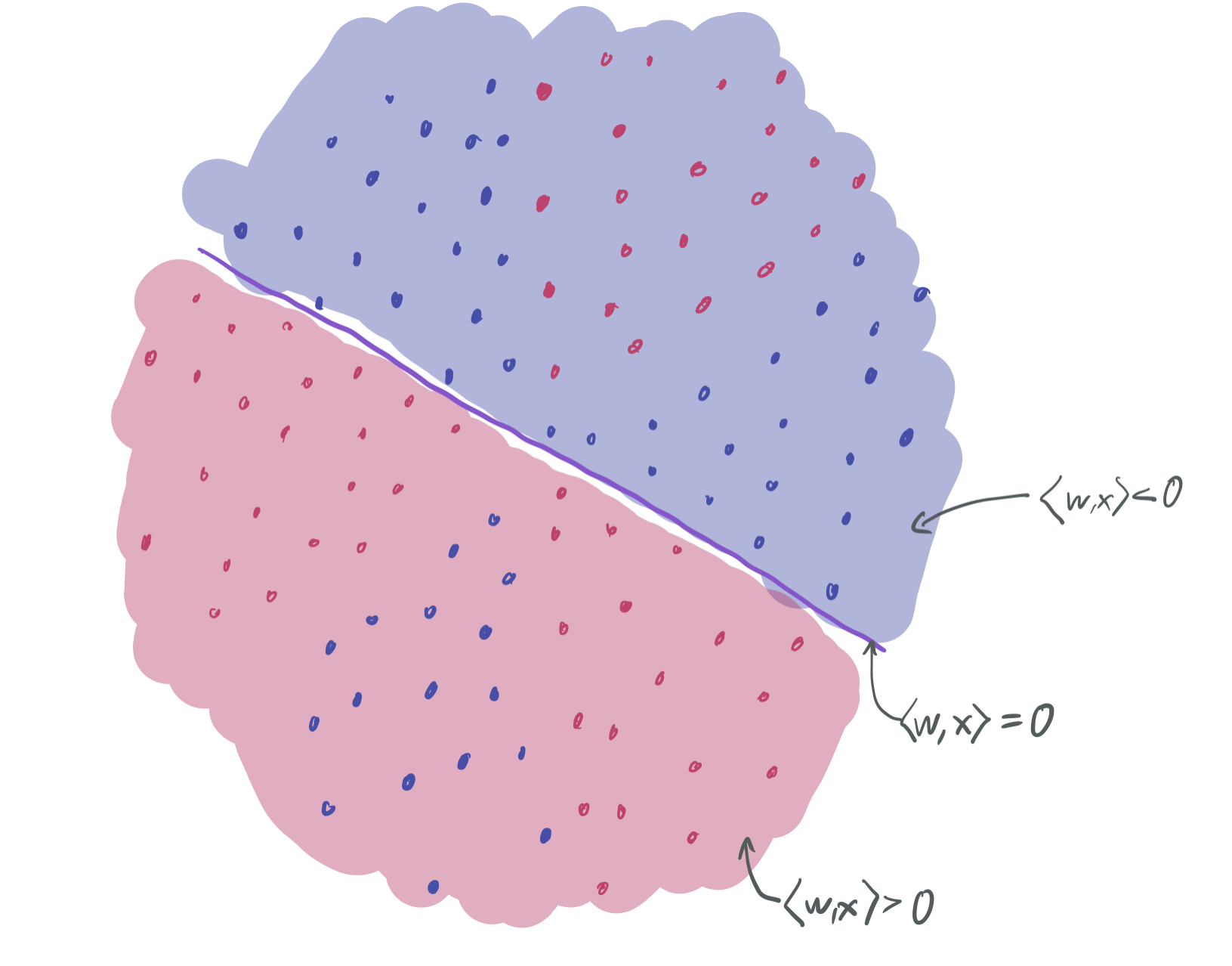
Neither of these are any good either.
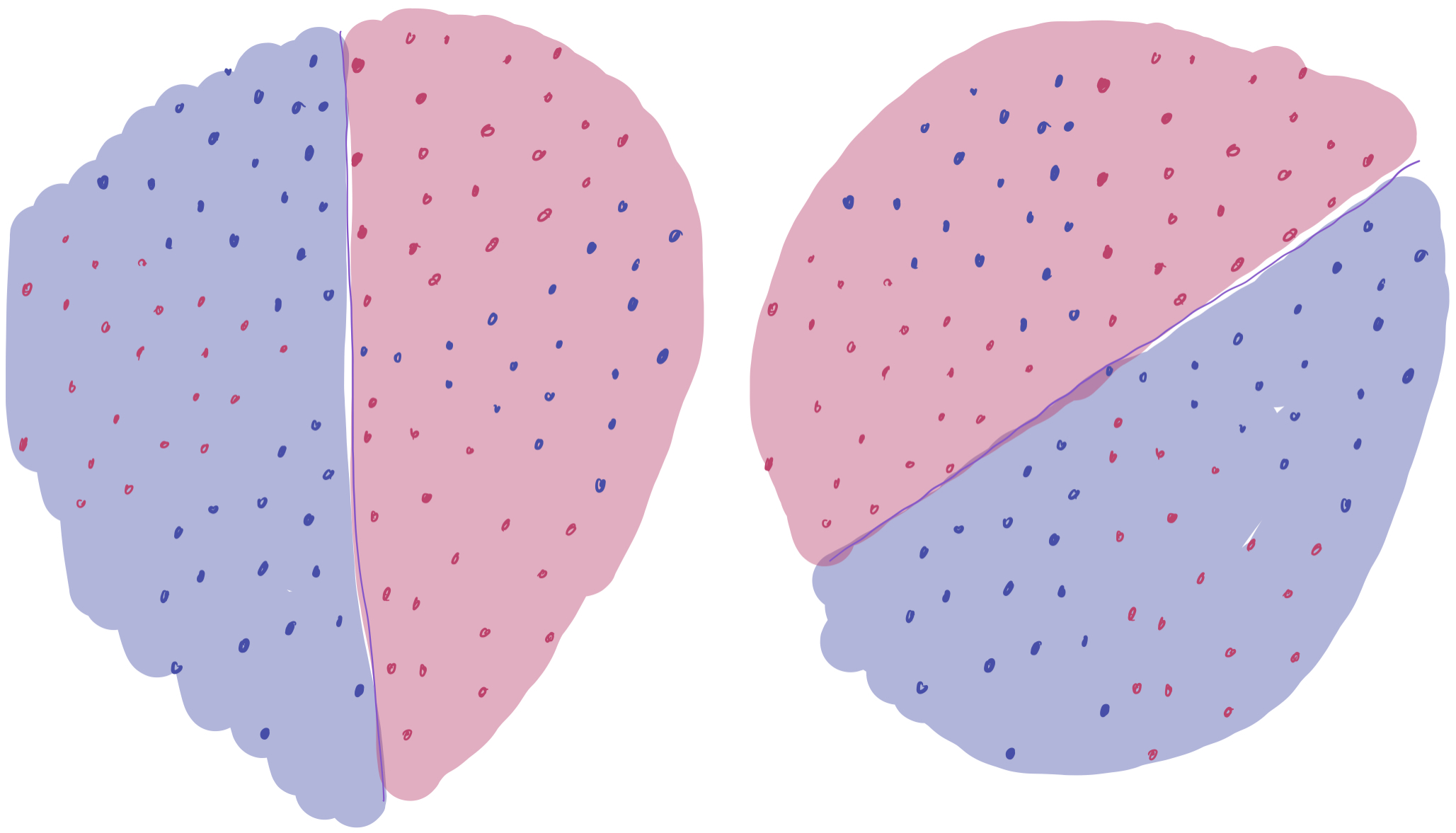
All three of the above linear separators have roughly a \(\frac23\) probability of classifying a sample correctly, but they each miss a different slice of the data. A natural question to ask is: Can these three separators be combined in some way to improve the training error of the classifier?
The answer is yes. By taking a majority vote of the three, one can correctly classify all of the data. That is, if at least two of the three linear classifiers think the point is red, then the final classifier predicts that the point is red. The following is a visualization of how this voting scheme works. (Maroon regions have 2 separators saying “red” and are classified as red. Purple regions have 2 separators saying “blue” and are classified as blue.)
We increase the complexity of the model (by aggregating together three different classifiers), which gets us down to zero training error in this case. This helps solve the issue about approximation–but it presents a new one on generalization. Can we expect this new “voting” classifier to perform well, since it’s more complex than just the linear classifier?
Boosting is an algorithm that formalizes this voting logic in order to string together a bunch of weak classifiers into one that performs well on all of the training data. In the last two sections of the blog post, we give two takes on generalization of boosting approaches, to answer the aforementioned question about whether we expect this kind of overfitting to hurt or not.
Weak Learners
The linear classifiers above are examples of weak learners, which perform slightly better than chance on the training data and which we combine together to make a stronger learner.
To formalize that concept, we say that a learning algorithm is a weak learning algorithm or a weak learner if it can PAC-learn a family of functions \(\mathcal{C}\) with error \(\epsilon = \frac12 - \eta\) with probability \(1- \delta\) where samples are drawn from some distribution \(\mathcal{D}\).
The idea with weak learning in the context of boosting is that you use the weak learning algorithm to obtain a classifier \(h\) that weak-learns the family over some weighted distribution of the samples. Then, the distribution can be modified accordingly, in order to ensure that the next weak learner performs well on the samples that the original hypothesis performed poorly on. In doing so, we gradually find a cohort of weak classifiers, such that each sample is correctly classified by a large number of weak learners in the cohort.
The graphic visualizes this flow. The top-right image represents the first weak classifier found on the distribution that samples evenly from the training data. It performs well on at least \(\frac23\) of the samples. Then, we want the weak learning algorithm to give another weak classifier, but we want it to be different and ensure that other samples are correctly classified, particularly the ones misclassified by the first one. Therefore, we amplify those misclassified samples in the distribution (bottom-left) and learn a new learning rule on that reweighted distribution. For that learning rule to qualify as a weak learner, it must classify \(\frac23\) of the weighted samples correctly. To do so, it’s essential that it correctly classifies the previously-misclassified samples. Hence, it chooses a different rule. Continuing to iterate this will give a wide variety of weak learners.
This intuition is formalized in the AdaBoost algorithm.
AdaBoost
Here’s how the algorithm works, as stolen from FS97.
- Input: some input set of samples \((x_1, y_1), \dots, (x_m, y_m)\), a number of rounds \(T\), and a procedure WeakLearn that outputs a weak learner given a distribution over samples.
- Initialize \(w^1 = \frac{1}{m} \vec{1} \in [0,1]^m\) to be a uniform starting distribution over training samples. (Note: the algorithm in the paper works for a general starting distribution, but we stick to the uniform distribution for simplicity.)
- For round \(t \in [T]\), do the following:
- Update the probability distribution by normalizing the current weight vector: \(p^t = \frac{1}{\|w^t\|_1} w^t.\)
- Use WeakLearn to obtain a weak learner \(h_t: X \to [-1,1]\).
- Calculate the error of \(h^t\) on the weighted training samples: \(\epsilon_t = \frac12 \sum_{i=1}^m p_i^t \lvert h_t(x_i) - y_i\rvert\). (Note: this differs by a factor of \(\frac12\) from the version presented in the paper because we assume the output of the functions to be \([-1,1]\) rather than \([0,1]\).)
- Let \(\beta_t = \frac{\epsilon_t}{1 - \epsilon_t} \in (0,1)\) inversely represent roughly how much weight should be assigned to \(h^t\) in the final classifier. (If \(h^t\) has small error, then it’s a “helpful” classifier that should be given more priority.)
- Adjust the weight vector by de-emphasizing samples that were accurately classified by \(h_t\). For all \(i \in [m]\), let
-
Output the final classifier, a weighted majority vote of the weak learners:
\[h_f(x) = \text{sign}\left(\sum_{t=1}^T h_t(x) \log\frac{1}{\beta_t} \right).\](This also differs from the final hypothesis in the paper because of the difference in output.)
This formalizes the process illustrated above, where we rely on WeakLearn to produce learning rules that perform well on samples that have been misclassified frequently in the past.
Why is it called AdaBoost? Unlike previous (less famous) boosting algorithms, it doesn’t require that all of the weak learners have minimum accuracy that is known to the algorithm. Rather, it can work with all errors \(\epsilon_t\) and hence adapt to the samples given.
It’s natural to ask about the theoretical properties of the algorithm. Specifically, can AdaBoost successfully aggregate a bunch of weak learners into a “strong learner” that classifies all but an \(\epsilon\) fraction of the training samples for any \(\epsilon\)? And if so, how many rounds \(T\) are needed? And how small must we expect \(\epsilon_t\) (the accuracy of each weak learner) to be? This leads us to the main AdaBoost theorem.
Theorem 1 [Performance of AdaBoost on training data, Theorem 6 of FS97]: Suppose WeakLearn generates hypotheses with errors at most \(\epsilon_1,\dots, \epsilon_T\). Then, the error of the final hypothesis \(h_f\) is bounded by
\[\epsilon \leq 2^T \prod_{t=1}^T \sqrt{\epsilon_t(1 - \epsilon_t)}.\]From this, one can naturally ask: How long will it take to classify all of the training data? For that to be the case, it suffices to show that \(\epsilon < \frac1m\), because there are only \(m\) samples and they cannot be “fractionally” correct.
For the sake of simplicity, we calculate the \(T\) necessary for \(\epsilon_t \leq 0.4\). (That is, each weak learner has advantage at least 0.1.)
\[\epsilon \leq 2^T \prod_{t=1}^T \sqrt{\epsilon_t(1 - \epsilon_t)} \leq 2^T (0.24)^{T/2} = (2 \sqrt{0.24})^T < \frac{1}{m},\]which occurs when
\[T > \frac{\log m}{\log (1 / (2 \sqrt{0.24}))} \approx 113 \log m.\]This is a really nice bound to have! It tells us that the training error can be rapidly bounded, despite only having the ability to aggregate classifiers that perform slightly better than chance.
The proof is simple and elegant, and I’m not going into it much. It’s well-explained by the paper, but much of it boils down to the intuition that if a training sample is neglected by many weak learners, then its emphasis continues to increase until it can no longer be ignored without meeting the weak learnability error guarantees.
Despite all of these nice things, this theorem is limited. It only covers the performance of the weighted majority classifier on the training data and says nothing about generalization. Indeed, it’s reasonable to fret about the generalization performance of this aggregate classifier. If we substantially increased the expressibility of the weak learning classifiers by combining them, then wouldn’t capacity-based generalization theory tell us that this will trade-off generalization? And isn’t it further compromised by the fact that training for a relatively small number of rounds leads to an aggregate hypothesis that perfectly fits the training data?
We focus for the remainder of the post on generalization, first examining it through the lens of classical capacity-based generalization theory, as done by FS97.
Capacity-based generalization
Looking back on the first visual of this post, classical learning theory has a simple narrative for what boosting does:
- The individual weak classifiers provided by WeakLearn lie on the left side of the curve (low generalization error, high training error) because they have a poor training error. Thus, they cannot fit complex patterns and are likely intuitively “simple,” which could translate to a low VC-dimension and hence a low generalization error.
- As each stage of the boosting algorithm runs, the aggregate classifier moves further to the right, improving training error at the cost of generalization error. After sufficiently many rounds \(T\) have occurred to drive the training error to zero, the generalization will be so large as to make any bound on population error vacuous.
This intuition is made explicit by the generalization bound presented by FS97, which bounds the VC-dimension of a majority vote of classifiers with individual VC-dimension at most \(d\) and applies the standard VC-dimension bound on generalization.
They get the following bound, which combines their Theorem 7 and Theorem 8.
Theorem 2 [Capacity-based generalization bound] Consider some distribution \(\mathcal{D}\) over labeled data \(X \times \{-1,1\}\) with some sample \(S\) of size \(m\) drawn from \(\mathcal{D}\). Suppose WeakLearn outputs hypotheses from a class \(\mathcal{H}\) having \(VC(\mathcal{H}) = d\). Then, with probability \(1 - \delta\), the following inequality holds for all final hypotheses that can returned by AdaBoost \(h_f\):
\[\text{err}_{\mathcal{D}}(h_f) \leq \underbrace{\text{err}_{S}(h_f)}_{\text{training error}} + \underbrace{O\left(\sqrt{\frac{dT\log(T)\log(m/dT) + \ln\frac1{\delta}}{m}}\right).}_{\text{generalization error}}\]This bound fits cleanly into the intuition described above. To keep the generalization small, \(T\) and \(d\) must be kept small relative to the number of samples. Doing so forces the training error to be large, because Theorem 1 suggests that \(h_f\) will have small training error when (1) AdaBoost runs for many iterates (large \(T\)) or (2) WeakLearn produces accurate classifiers, which requires an expressive family of weak learners (large \(d\)). Hence, we’re necessarily trading off the two types of error.
However, this isn’t the full story. When running experiments, they confirmed that after many rounds, the training error approached zero (as expected by Theorem 1). But they also found that the test error dropped along with the training error and that the test error continued to drop even after the training error went to zero. To explain this phenomenon, we turn to BFLS98, where the authors explain this low generalization error using margin-based bounds rather than capacity-based bounds.
Margin-based generalization
A key idea in the story about margin-based generalization is that a classifier that correctly and decisively categorizes all the training data is more robust (and more likely to generalize) than one that nearly categorizes samples incorrectly. Roughly, slightly perturbing the samples in the first case will lead to samples that have the same labels, while that may not be the case in the second case.
Analyzing this requires considering some notion of margin, which quantifies the decisiveness of the classification. For now, consider a modified version of the weighted majority classifier derived from AdaBoost:
\[h_f(x) = \sum_{t=1}^T h_t(x) \log\frac{1}{\beta_t}.\]The only difference here is that we dropped the \(\text{sign}\) function, which means the output may be anywhere in \([-1,1]\). \(h_f\) categorizes the sample \((x,y)\) correctly if \(yh_f(x) > 0\), because the sign of \(h_f\) will then match \(y\). We say that \(h_f\) categorizes a sample correctly with margin \(\theta > 0\) if \(yh_f(x) \geq \theta\). This means that–if \(h_f\) is an aggregation of a large number of weak classifiers–then a small number of those classifiers changing their outcomes will not change the overall outcome of \(h_f\).
There are two key steps that lead to new generalization bounds by BFLS98 for AdaBoost.
- AdaBoost (after sufficiently many rounds \(T\) and with sufficiently small weak learner errors \(\epsilon_t\)) will classify the sample \(S\) correctly with some margin \(\theta\).
- Any linear combination of \(N\) classifiers (each of which has bounded VC dimension) with margin \(\theta\) on the training data has a generalization bound that depends on \(\theta\) and not on \(N\).
They accomplish (1) by proving a theorem that is very similar in flavor and proof to the Theorem 1 we gave earlier.
Theorem 3 [Margins of AdaBoost on training data, Theorem 5 of BFLS98]: Suppose WeakLearn generates hypotheses with errors at most \(\epsilon_1,\dots, \epsilon_T\). Then, the final hypothesis \(h_f: X \to [-1,1]\) satisfies the following margin bound on the training set \((x_1, y_1), \dots, (x_m, y_m)\) for any \(\theta \in [0,1)\):
\[\frac1{m} \sum_{i=1}^m \mathbb1\{y_ih_f(x_i) \leq \theta \}\leq 2^T \prod_{t=1}^T \sqrt{\epsilon_t^{1-\theta}(1 - \epsilon_t)^{1 + \theta}}.\]To make matters more concrete once again, consider the case where \(\epsilon_t \leq 0.4\) as before. Then, the bound gives
\[\frac1{m} \sum_{i=1}^m \mathbb1\{y_ih_f(x_i)\leq \theta\} \leq 2^T (0.4)^{T(1- \theta)/2} (0.6)^{T(1 + \theta)/2}.\]If we want all training samples to obey the condition, we enforce that the margin term is less than \(\frac1{m}\). Consider two cases:
- By some calculations (with the help of WolframAlpha), if \(\theta = 0.1\), then \(y_i h_f(x_i) \geq \theta\) for all \(i \in [m]\) if \(T > 7260 \log m\). This is very similar to our application of Theorem 1, albeit with bigger constants.
-
If \(\theta = 0.2\), then
\[2^T (0.4)^{T(1- \theta)/2} (0.6)^{T(1 + \theta)/2} = 2^T (0.4)^{0.4T}(0.6)^{0.6T} \approx 1.02^T,\]which means that the bounds can never guarantee that the margins will be that large with time.
These bounds provide a way of finding a margin \(\theta\) dependent on \(T\) and errors \(\epsilon_1, \dots, \epsilon_T\), which will be useful in the second part.
To get (2), they prove a bound on the combination of weak learners with margin bounds.
Theorem 4 [Margin-based generalization; Theorem 2 of BFLS98]: Consider some distribution \(\mathcal{D}\) over labeled data \(X \times \{-1,1\}\) with some sample \(S\) of size \(m\) drawn from \(\mathcal{D}\). Let \(\mathcal{H}\) be a family of “base classifiers” (weak learners) with \(VC(\mathcal{H}) = d\). Then, with probability \(1 - \delta\), any weighted average \(h_f(x) = \sum_{j=1}^T p_j h^j(x)\) for \(p_j \in [0,1]\), \(\sum_j p_j = 1\), and \(h^j \in \mathcal{H}\) satisfies the following inequality:
\[\text{err}_{\mathcal{D}}(h_f) = \text{Pr}_{\mathcal{D}}[y h_f(x) \leq 0] \leq \frac1{m} \sum_{i=1}^m \mathbb1\{y_ih_f(x_i)\leq \theta\} + O\left(\sqrt{\frac{d \log^2(m/d)}{m\theta^2} + \frac{\log(1/\delta)}{m}}\right).\]This is fantastic compared to Theorem 2 because the generalization bound does not worsen as \(T\) increases. The opposite effect actually occurs: as AdaBoost continues to run, Theorem 3 shows that the margin increases (up to a point), which strengthens the bound without trade-off!
We can instantiate the bound in the setting described above to show what a nice generalization bound can look like for boosting. If, once again, \(\eta_t \leq 0.4\), then taking \(\theta = 0.1\) and \(T = 7260\log m\) gives
\[\text{err}_{\mathcal{D}}(h_f) = O\left(\sqrt{\frac{d \log^2(m/d) + \log(1/\delta)}{m}} \right).\]In this case, we can have our cake and eat it too; we increase the model complexity and expressivity by increasing \(T\), but we don’t sustain the basic trade-offs between training and generalization error discussed at the beginning of the post.
To illustrate why, we give a high-level overview of the proof and show how the rough intuition that “decisive classification leads to robustness, leads to generalization” holds up.
- The proof uses an approximation of \(h_f = \sum_{j=1}^T p_j h^j\) by sampling \(N\) classifiers \(\hat{h}_1, \dots, \hat{h}_N\) independently from \(h^1, \dots, h^T\) weighted by \(p_1, \dots, p_T\). It averages them together to obtain \(g = \frac1{N} \sum_{k=1}^N \hat{h}_k.\)
-
The proof decomposes the population error term into other quantities by using properties of conditional probability:
\[\text{Pr}_{\mathcal{D}}[y h_f(x) \leq 0] \leq \text{Pr}_{\mathcal{D}}\left[y g(x) \leq \frac{\theta}{2}\right] + \text{Pr}_{\mathcal{D}}\left[y g(x) \leq \frac{\theta}{2}, y h_f(x) \leq 0\right].\] - The second term can be shown to be small when \(N\) and \(\theta\) large with high probability over \(g\) by a Chernoff bound. Since \(h_f = \mathbb{E}[g] = \mathbb{E}[\hat{h}_k]\), it’s unlikely that \(yg(x)\) and \(yh_f(x)\) will differ by a large factor from one another.
- By principles of VC dimension, the Sauer-Shelah lemma, and concentration bounds (this time over the sample) for large \(m\), the first term will be roughly the same as \(\frac1{m} \sum_{i=1}^m \mathbb{1}\{ y_i g(x_i) \leq \theta / 2 \}.\)
-
Using the same conditional probability argument as before, that same term can be decomposed into
\[\frac1{m} \sum_{i=1}^m \mathbb{1}\{ y_i g(x_i) \leq \theta / 2 \} \leq \frac1{m} \sum_{i=1}^m \mathbb{1}\{ y_i f(x_i) \leq \theta \} + \frac1{m} \sum_{i=1}^m \mathbb{1}\{ y_i g(x_i) \leq \theta / 2 , y_i f(x_i) \leq \theta\}.\] - Using Chernoff bounds shows the second term of the expression is small with high probability over \(g\). Thus, the \(\text{Pr}_{\mathcal{D}}[y h_f(x) \leq 0]\) is approximately \(\frac1{m} \sum_{i=1}^m \mathbb{1}\{ y_i g(x_i) \leq \theta / 2 \}\), plus an error term that accumulates as a result of the concentration bounds.
- Having a large \(\theta\) means that we have plenty of room for the Chernoff bounds over \(g\) to be strong, which corresponds to the robustness discussed before. If \(\theta\) were small, then it would be very easy to have \(yf(x) \leq 0\) and \(yg(x) \geq \theta/2\) simultaneously, which would make the argument impossible.
Last thoughts
I read these boosting papers in 2017 while taking my first graduate seminar, which surveyed a variety of papers in ML theory. I enjoyed the papers then, but the remarkability of this generalization result was lost on me at the time. Now, I find this much more exciting because it gives a setting where a model can obtain provably great generalization error despite overfitting the data and being “over-parameterized.” (If we count the number of parameters used in all of the classifiers that vote, there can be many more parameters than samples \(m\).) The proof is elegant and does not require strange and adversarial distributions over training data. Granted, the assumption that there exists a weak learner that always returns a classifier with error at most (say) 0.4 is a strong one, but the result is remarkable nonetheless.
Thanks for reading! Leave a comment if you have any thoughts or questions. (As long as the comments system isn’t buggy on your end–I’m still sorting out some issues.) See you next time!
Comments