What does the 'R-norm' reveal about efficient neural network approximation? (COLT 2023 paper with Navid and Daniel)
[technical research learning-theory Well, in the paper summary I posted last year, I promised more posts, none of which materialized. So I won’t promise anything this time around; I enjoy writing these posts, but it’s hard to find the time with all of the other grad school and life things going on.
Anyways, here goes another paper summary on a work that is published at this year’s COLT in Bangalore (!!). A big reason for writing this post is to explain the “story” of the paper in as clear a way as possible, without getting too bogged down in the technical details. (Note the time gap between when we posted the paper on arXiv and its publication in July at COLT. Needless to say, it took us a while to figure out the right way to tell the story.)
Quantifying efficient approximation: width vs weight norm
As I’ve discussed in a past summary, we can consider three rough mathematical problems about deep learning theory: approximation (what types of mathematical functions can be represented by neural networks), optimization (how gradient-based learning algorithms converge to neural networks that fit the training data), and generalization (how a trained network performs on never-before-seen data).
If we focus on approximation, the first question one asks is whether there exists a neural network that approximates a function, and the answer to that is almost always yes, due to famous universal approximation results. The second question to ask is whether there exists a reasonably sized neural network that approximates the function. This question yields more nuanced results, with a wealth of positive and negative results, but its answers hinge on how we define “reasonably sized.”
The typical approach is to quantify the size of a neural network by the size of the graph needed to compute it: that is, by the number of neurons, its width, or its depth. This shows itself in my past work on universal approximation, as well as well-known depth-separation papers (e.g. Telgarsky16, ES16, Daniely17). In these works, we regard a two-layer neural network
\[g(x) = \sum_{i=1}^m u^{(i)} \sigma(\langle w^{(i)}, x\rangle + b^{(i)})\]with ReLU activations (\(\sigma(z) = \max(0, z)\)) as an efficient approximation of some function \(f\) if \(\|f - g\|\) is small (with respect to some norm, possibly \(L_2\) over some distribution or \(L_\infty\)) and if the width \(m\) is bounded, specifically if \(m = \mathrm{poly}(d)\) for input dimension \(d\) (i.e. \(x \in \mathbb{R}^d\)).
However, this focus on width is not without its drawbacks. The primary drawback is that even if a low-width solution exists, there’s no guarantee gradient descent will find it. (Note that when we talk about the bias of a learning algorithm, we’re talking about how it breaks ties. Since we often live in the over-parameterized regime, there are generally many different networks that attain zero training loss. The bias of the algorithm determines how the learning algorithm selects one.) More generally, it’s not even apparent that gradient descent should be biased in favor of low-width solutions. Since we train neural networks by making continuous weight updates rather than “pruning” neurons (by setting specific weights \(u^{(i)} = 0\) algorithmically), it’s unlikely that it will converge exactly to a low-width network if such an approximation exists.
So if not width, how can we quantify efficient approximation? One alternative approach, given in this paper by Saverese, Evron, Soudry, and Srebro, is to instead quantify neural network size by the norm of its weights. The \(\mathcal{R}\)-norm quantity proposed by SESS is roughly
\[\|g\|_{\mathcal{R}} = \| w\|_2^2 + \| u \|_2^2 = \sqrt{\sum_{i=1}^m (u^{(i)2} + \| w^{(i)} \|_2^2)}.\]If we assume that each weight vector satisfies \(\|w^{(i)}\|_2 = 1\) (which we can safely do because the ReLU activation is homogeneous; we can normalize \(w\) while scaling \(w\) and \(b\) accordingly and preserve the same network output), then we can simplify the expression to be
\[\|g\|_{\mathcal{R}} = \| u \|_1.\]The definition of \(\mathcal{R}\)-norm is a little more technical; check out our paper to see how we define two slightly different variants of the norm. Notably, our formulation of the R-norm doesn’t count bias terms \(b^{(i)}\), to the chagrin of some researchers.
Given this description, we only care about the width \(m\) in as much as it increases the the \(\mathcal{R}\)-norm of the network; this framing rules out the above concern of a low-width high-weight solution that gradient descent struggles to converge to, while opening the possibility of a very high width (or even infinite-width) neural network with small weight neurons.
Why use this \(\mathcal{R}\)-norm minimizing framing? For one, it fits nicely with studies of explicit regularization of both neural networks and other models. When learning linear models of the form \(x \mapsto w^T \phi(x)\) for feature mapping \(\phi: \mathbb{R}^d \to \mathbb{R}^m\), it’s easy to regularize the target function by adding a norm penalty to \(w\). If the goal is to rely on a small number of the \(m\) features stipulated by \(m\), then adding an \(\ell_1\) penalty term will likely be more effective than some kind of more direct feature pruning approach. Neural networks often are trained with explicit regularization of the norms of their weights, providing a direct incentive to find a low-norm function that fits the data. Moreover, there’s evidence that gradient descent has an implicit bias in favor of low-norm solutions; see papers like this one.
Our key question: understanding \(\mathcal{R}\)-norm minimizing interpolation
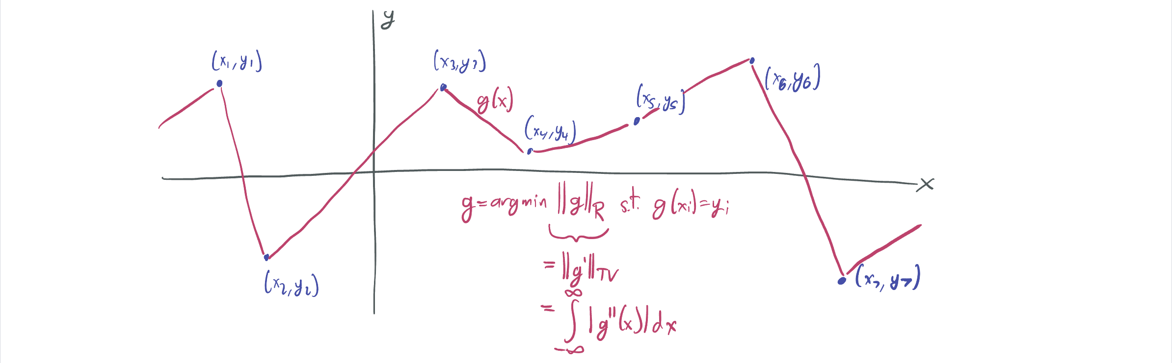
This brings us to our key question: What are the properties of the two-layer neural network \(g\) that perfectly fits a dataset while minimizing the R-norm? For a given dataset \(\mathcal{D} = \{(x_i, y_i) \in \mathbb{R}^d \times \mathbb{R}\}\), we characterize solutions to the variational problem (VP)
\[\inf_{g} \|g\|_{\mathcal{R}} \text{ s.t. } g(x_i) = y_i \ \forall i \in [n],\]or to the \(\epsilon\)-variational problem
\[\inf_{g} \|g\|_{\mathcal{R}} \text{ s.t. } |g(x_i) - y_i| \leq \epsilon \ \forall i \in [n].\]We’re not the first group to ask this question:
- SESS showed that when \(d = 1\), the \(\mathcal{R}\)-norm minimizing network \(g\) fitting the dataset is the one whose derivative has minimum total variation, which is satisfied by a piecewise-linear spline interpolation of the dataset.
 Subsequent work by Hanin exactly characterizes this one-dimension interpolation regime.
 - A paper by Ongie, Willets, Soudry, and Srebro characterizes the general \(d\)-dimensional case by relating the \(\mathcal{R}\)-norm to a norm based on the Radon transform, which bounds the total ReLU weight needed to represent a function \(f\) by expressing \(f\) as the as a bunch of integrals over subspaces with different angles. (Think: x-rays, where an scan can be computed by firing a bunch of individual beams through a body at different angles.) (Image below is from OWSS.)
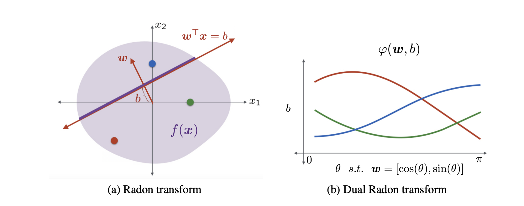 While this equivalence holds, its primary implications are impossibility results (e.g. that two layer networks cannot efficiently represent certain radial functions) rather than quantitative insights into how certain datasets are fit.
We decided to focus on a higher-dimensional analogue of (1) that provides more concrete quantitative results than (2), while sacrificing some generality. We did so by focusing on a particular dataset and showing that the solution to its VP is somewhat unexpected.
Our specific questions on interpolating parities
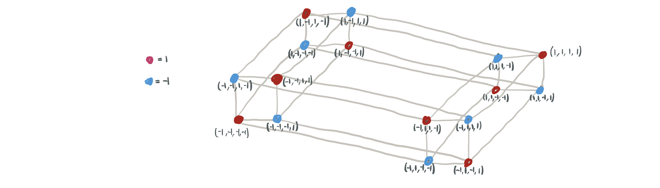
The dataset is the parity dataset, \(\mathcal{D} = \{(x, \chi(x)): x \in \{\pm 1\}^d\}\), where \(\chi: x \in \{\pm 1\} \mapsto \prod_{j=1}^d x_j \in \{\pm1\}\), illustrated below for \(d = 4\).
 Why this one?
- It’s a \(d\)-dimensional function, and every input has significant bearing on the output; flipping a single bit of \(x\) will flip the entire output of \(\chi\).
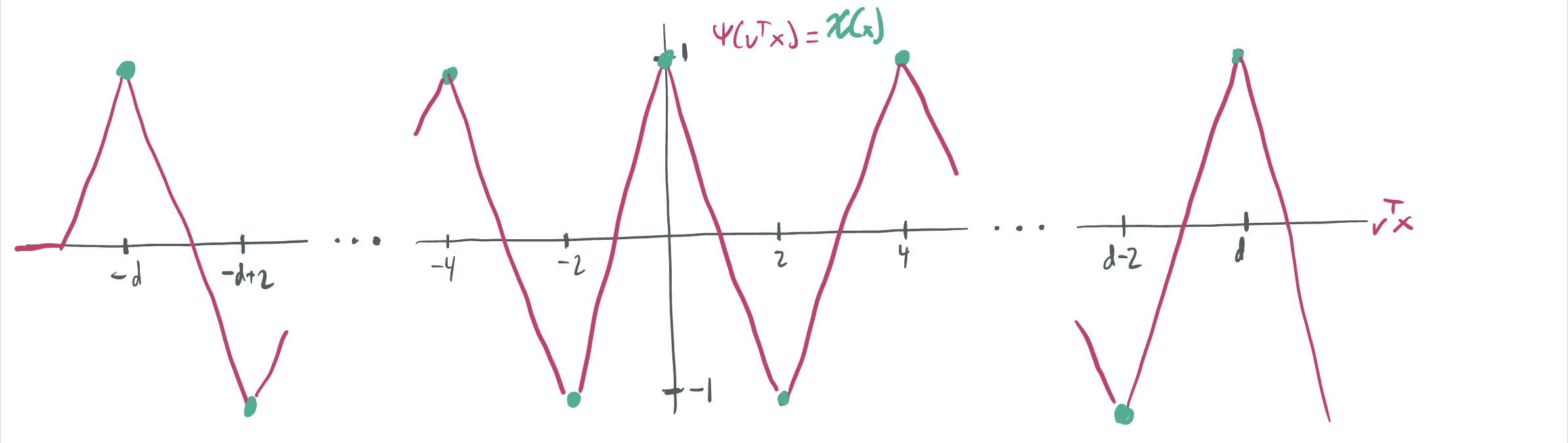
- Yet, it has a “low intrinsic dimensionality.” \(\chi\) is a ridge function, which means that there exists some \(v \in \mathbb{R}^d\) and \(\psi: \mathbb{R} \to \mathbb{R}\) such that \(\chi(x) = \psi(v^T x)\). That is, there exists a one-dimensional input projection that exactly determines the output.
- For parity, there are \(2^d\) possible choices of \(v\): any vector in \(\{\pm 1\}^d\). This follows from the fact that \(\chi\) is symmetric up to bit flips: \(\chi(v \odot x) = \chi(v) \chi(x)\).
- The scalar function \(\psi: \mathbb{R} \to \mathbb{R}\) is a sawtooth function, which oscillates \(O(d)\) times between \(-1\) and \(1\).
The “ridgeness” of the dataset is central to the motivation. Learning such functions with gradient descent is well-studied (including by a paper by yours truly with some collaborators at NYU). Neural networks trained in the feature learning regime have substantial generalization advantages on inputs labeled by intrinsically-low dimensional targets.
Learning parity functions (specifically, given a dataset \(\{(x_i, y_i)\}_{i \in [n]}\), trying to find a subset of variables \(S \subset [n]\) such that \(\chi_S(x) = \prod_{j \in S} x_j\) best describes the dataset) is a well-known and difficult learning problem, for both neural networks and general ML theory approaches. While parity can be learned in the noiseless case (where always \(y_i = \chi_S(x_i)\)) using Gaussian elimination using \(n = d\) samples, it’s considered a hard problem in the noisy setting (where a small fraction have flipped labels), and it’s the classic example of a learning problem with a high statistical query complexity. (See last year’s post for a brief intro to SQ.) Gradient-based algorithms for learning even sparse parities (where \(|S| \ll d\)) with neural networks are computationally intensive, as is illustrated by this paper among others.
There are two major questions we study about this dataset:
- [Approximation] What is the intrinsic dimensionality of the \(\mathcal{R}\)-norm minimizing interpolation of the dataset labeled by \(\chi\)? Specifically, since the data can be labeled by some ridge function, is the network \(g\) a ridge function as well?
- [Generalization] What is the sample complexity of learning noiseless parities labeled by \(\chi_S\) for unknown \(S \subset [n]\) using \(\mathcal{R}\)-norm minimization as a learning algorithm?
Question 1: What’s the most efficient approximation?
When we first started thinking about this problem, our first thought was that a ridge dataset of this form would have the same message as the SESS and Hanin papers: \(g\) would take the form of a ridge function \(g(x) = \phi(v^T x)\) that performs linear spline interpolation on the samples. (For simplicity, let’s assume that \(d\) is even.)
Given the properties of parity discussed above, a reasonable guess is that that’ll be attained by the sawtooth interpolation \(g(x) = \psi(v^T x)\). To write this as a neural network in the desired form, we take \(v = \vec{1} = (1, \dots, 1)\) and let
\[g(x) = \sqrt{d}\sigma\left(\left\langle \frac{\vec1}{\sqrt{d}}, x \right\rangle + \frac{d+1}{\sqrt{d}}\right) - 2\sqrt{d}\sum_{j=0}^d (-1)^j \sigma\left(\left\langle \frac{\vec1}{\sqrt{d}}, x \right\rangle + \frac{d - 2j}{\sqrt{d}}\right).\]We visualization the ReLU construction of the sawtooth as blue and purple curves, added up to make full red sawtooth.
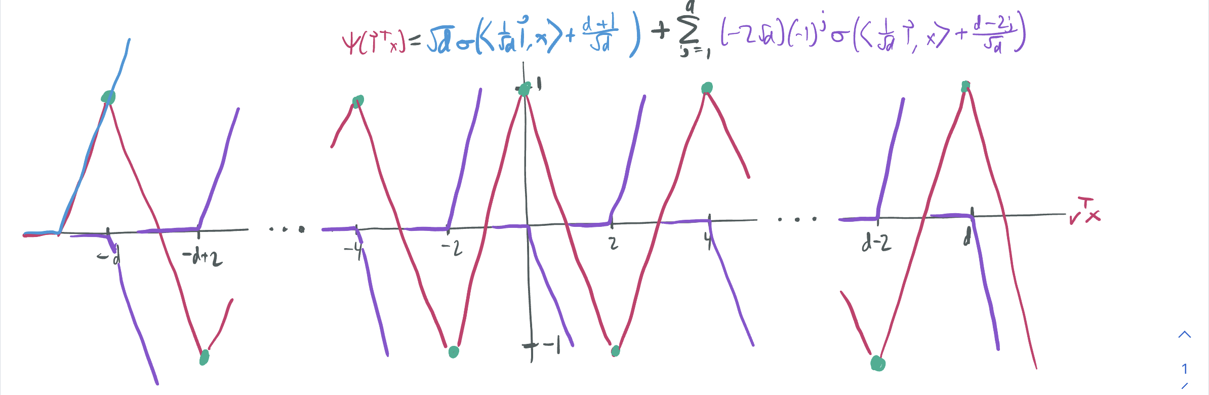
We can verify that (1) this is a valid 2-layer neural network with unit-norm weight vectors \(\vec1 / \sqrt{d}\), (2) the single ReLU outside of the sum ensures that \(g(-\vec1) = (-1)^d = 1\), and (3) the sum of alternate-sign ReLUs ensures causes more to activate as as the inner product \(\langle \vec1, x\rangle\) increases and ensures that \(g(x) = \chi(x)\) everywhere else. Then, we can compute the \(\mathcal{R}\)-norm by computing the \(\ell_1\) norm of the top layer weights:
\[\|g\|_{\mathcal{R}} = \sqrt{d} + (d+1) \cdot 2 \sqrt{d} = O(d^{3/2}).\]With the benchmark of an \(\mathcal{R}\)-norm of \(d^{3/2}\), we can then ask about its optimality.
First follow-up: Can we do better with other ridge functions?
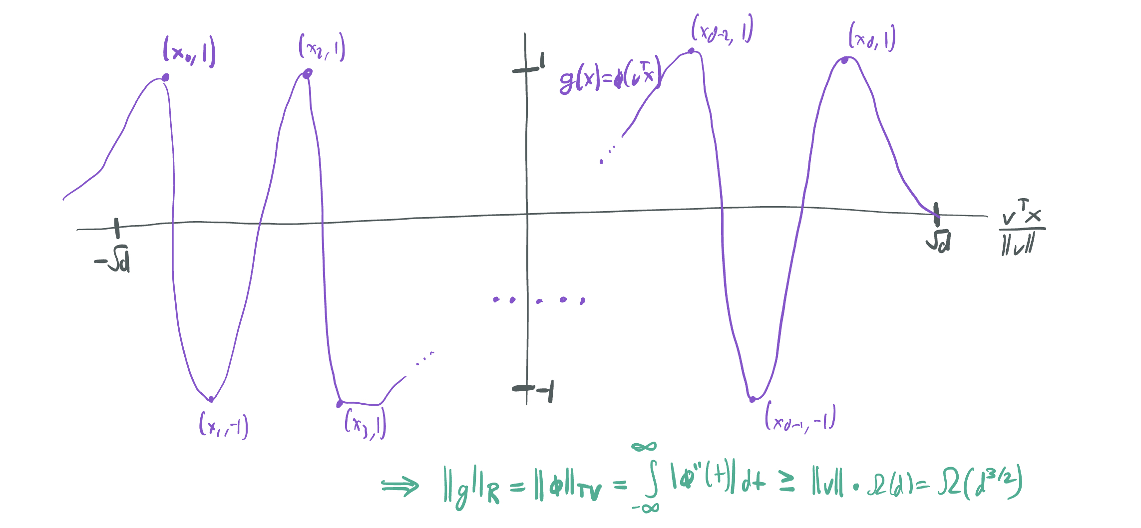
That is, is there some other \(g(x) = \phi(v^T x)\) having \(\|g\|_{\mathcal{R}} = o(d^{3/2})\)?
Theorem 3 of our paper shows that we cannot do better with another ridge function. It relies on the key fact proven by SESS: that when \(g\) is a ridge function, \(\|g\|_{\mathcal{R}} = \int_{-\infty}^\infty |\phi''(z)| dz\). While the second derivative does not exist for functions like \(\phi\) composed of ReLU activations, we can circumvent the problem by noting that the total variation of \(\phi'\) can also be lower-bounded by showing that \(\phi\) must oscillate a certain number of times on a sufficiently short interval. It then suffices to show that for any choice of \(v \in \mathbb{R}^d\), \(g\) would have to oscillate between \(-1\) and \(1\) at least \(d\) times on an interval length at most \(\sqrt{d}\). We accomplish this by picking a direction \(w\), selecting a subset of \(d+1\) samples oriented in that direction with alternating sign outputs, and using the mean value theoremt to show that the derivative of \(\phi\) must take on alternately large and small values as well.
Second follow-up: Can we do better with any other functions, if they aren’t ridge?
This part came as a surprise to us; we initially thought that the ridge was the best possible solution, but it turns out there’s a way to do better by sacrificing width and taking advantage of the symmetry of the partiy function.
In Theorem 4, we show that there exists a neural network \(g\) having \(\|g\|_{\mathcal{R}} = O(d)\) that perfectly fits the dataset. We construct \(g\) to be a function of width \(O(2^d)\) that averages together “single-bladed sawtooths” in each of the \(2^d\) directions:
\[g(x) = \frac{Q}{2^d} \sum_{v \in \{\pm 1\}^d} \chi(x) s(v^T x),\]where \(s(z)\) is a piecewise linear function with \(s(0) = 1\) and \(s(z) = 0\) for \(\lvert z\rvert\geq 1\) that can be represented with three ReLUs and \(Q\) is a normalization quantity to be fixed later.
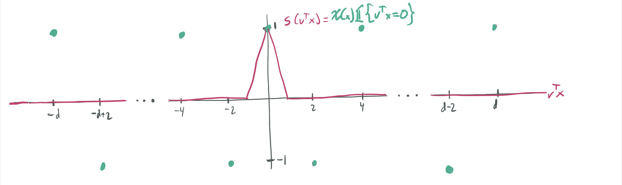 The key insight is that each \(s(v^T x)\) has an \(\mathcal{R}\)-norm of \(O(\sqrt{d})\) and will correctly label a roughly \(\frac1{\sqrt{d}}\) fraction of all inputs.
(For intuition, note that that the probability of a \(\mathrm{Bin}(n, \frac12)\) random variable returning \(\frac{n}2\) is also roughly \(\frac1{\sqrt{d}}\).)
Then, we can let \(Q = \Theta(\sqrt{d})\), which ensure that \(\|g\|_{\mathcal{R}} = O(d)\).
The key insight is that each \(s(v^T x)\) has an \(\mathcal{R}\)-norm of \(O(\sqrt{d})\) and will correctly label a roughly \(\frac1{\sqrt{d}}\) fraction of all inputs.
(For intuition, note that that the probability of a \(\mathrm{Bin}(n, \frac12)\) random variable returning \(\frac{n}2\) is also roughly \(\frac1{\sqrt{d}}\).)
Then, we can let \(Q = \Theta(\sqrt{d})\), which ensure that \(\|g\|_{\mathcal{R}} = O(d)\).
If the gap between this construction and the full sawtooth ridge construction is surprising, here’s a little bit of intuition. We can think of any ReLU in the construction as a having a “cost” according to its coefficient \(u^{(i)}\), and our aim is to have a low ratio of cost the ratio of the dataset that is perfectly fit due to the existence of the ReLU.
- Since a \(\frac{1}{\sqrt{d}}\) fraction of the samples have \(v^T x = 0\) for any fixed \(v \in \{\pm q\}^d\), the all of the ReLUs used to construct the “averaged single sawthooths” construction is cost-efficient.
- Due to basic binomial concentration, an exponentially small fraction of samples have \(\lvert\vec{1}^T x\rvert \geq C\sqrt{d}\). This means that \(d - C\sqrt{d}\) of the ReLUs in the sawtooth ridge construction have the same high cost as the others, but cause extremely few samples to be perfectly fit.
Thus, the magic of the averaging construction comes from the fact that we’re getting maximum usage out of each ReLU.
Note: In case the high width of the construction is offputting, we have a construction for the \(\epsilon\)-approximate variational problem in Theorem 5 with width \(m = \tilde{O}(d^{3/2} /\epsilon^2)\).
Third follow-up: Is \(O(d)\) the best possible \(\mathcal{R}\)-norm for parity interpolation?
Theorem 6 of our paper concludes that this is the case: any \(g\) that even approximates the dataset to accuracy \(\frac12\) over \(L_2\) distance must have \(\mathcal{R}\)-norm at least \(\frac{d}{16}\). The main step of the proof places an upper bound on the maximum correlation any single ReLU neuron can have with \(\chi\).
Taken together, these results provide a clear quantitative separation on the parity dataset between the suboptimality of the representational cost of using ridge functions to approximate the parity dataset.
- \(\inf\{\|g\|_{\mathcal{R}}: g(x_i) = y_i \ \forall i \in [n]\} = \Theta(d)\).
- \(\inf\{\|g\|_{\mathcal{R}}: g(x_i) = y_i \ \forall i \in [n], \ g(x) = \phi(v^T x)\} = \Theta(d^{3/2})\).
Are we too fixated on parity?
Maybe you think this is cool, but maybe you’re also concerned about the dependence on the parity dataset. After all, the parity function has all kinds of crazy symmetries gives \(2^d\) different symmetric sawtooth functions achieving optimal \(\mathcal{R}\)-norms among ridge functions. Why shouldn’t there be something strange going on?
We had those concerns too, so we developed Section 5 of the paper as well, which translates several of the results to more generic sinusoidal functions on \(\{\pm 1\}^d\). For these datasets, there’s no such symmetry, and there’s a much more natural ridge interpretation in the single direction of lowest frequency. And yet, an average of truncated sawtooths of varying frequency is still the optimal thing to do. To us, this presents a fundamental tradeoff in efficient representation between low intrinsic dimensionality and averaging together partial solutions.
Question 2: Can \(\mathcal{R}\)-norm minimization learn parities?
So far, we’ve thought about solving the variational problem on a dataset that labels all \(2^d\) points of the form \((x, \chi(x))\). Now, we shift our interest towards learning \(\chi_S\) given \(n\) independent samples \(\mathcal{D} = \{(x_i, \chi_S(x_i)): i \in [n]\}\) with \(x_i\) drawn uniformly from \(\{\pm 1\}\). This is a more traditional learning setting, where the learning algorithm chooses the neural network \(g\) that solves the variational problem on \(\mathcal{D}\).
In a sense, we’re trying to analyze neural networks while avoiding analyzing gradient descent (which can be oh so ugly). If we assume that our gradient-based optimization method (either due to explicit regularization or inductive bias) convergence to the \(\mathcal{R}\)-norm minimizing interpolant, then we can assess its success at learning parities.
Note that we’ve now shifted our orientation from approximation to generalization. The best possible sample complexity \(n\) we can hope for is \(n = O(d)\), since Gaussian elimination cannot be beaten for noiseless parities.
The positive result
Theorem 9 of our paper shows that with \(n = O(d^3 / \epsilon^2)\) samples, then the solution \(g\) to the variational problem (with an appended “clipping function” that reduces its outputs to the interval \([-1, 1]\)). This is a pretty straight-forward bound that relies on Rademacher complexity techniques. We’re able to characterize expressive capacity of the family of functions produced by solving the variational problem by taking advantage of the fact that their norms are bounded. From there, the derivation of generalization bounds follow standard ML techniques.
The negative result
On the other hand, Theorem 7 suggests that \(\mathcal{R}\)-norm minimizing interpolation will fail with substantial problem any time \(n \ll d^2\). This means that the learning algorithm—while it still works for a polynomial number of samples—is suboptimal in terms of sample complexity. What we prove is actually stronger than that: the \(L_2\) distance between the network \(g\) and any parity function will be nearly 1, which means that there’s no meaningful correlation between the two.
This result is a bit more methodologically fun, mainly because it draws on our approximation-theoretic results.
- We construct a neural network \(h\) that perfectly fits \(n \leq d^2\) random samples that has \(\|h\|_{\mathcal{R}} = \tilde{O}(n / d)\). This uses the same construction as a low-Lipschitz neural network presented by Bubeck, Li, and Nagaraj, which uses a single ReLU to fit each individual sample. With high probability, each of these ReLUs is active for at most one sample and has a low-weight coefficient.
- This means that solving the variational problem must return a network \(g\) with \(\|g\|_{\mathcal{R}} \leq \tilde{O}(n / d)\).
- However, our Theorem 6 implies that if \(\|g\|_{\mathcal{R}} \ll d\), then it can’t even correlate with parities \(\chi_S\) for \(\lvert S\rvert = \Theta(d)\). Hence, if \(n \ll d^2\), we have no hope of approximating parity from the \(n\) samples.
What about the gap?
We have both upper and lower bounds, but the story is not complete, since there’s a \(d^2\) vs \(d^3\) gap on the minimum sample complexity needed to learn with \(\mathcal{R}\)-norm minimization. We’re not sure if there’s a nice way to close the gap, but we think it’s worth noting that the BLN paper itself has studies an open question about the minimum-Lipschitz network of bounded width that fits some samples. The construction we draw on in the proof of our negative result might be suboptimal, in which case we might be able to lift our \(d^2\) bound with a more efficient construction.
Where does this leave us?
So that’s the summary of this slightly strange paper, which considers generalization and approximation of a very specific learning problem on neural networks with a very specific kind of regularization. This work ties in tangentially to several different avenues of neural network theory research: inductive bias, approximation separations, adaptivity, parity learning, ensembling, and intrinsic dimensionality. Our intention was to elucidate the tension between optimizing for low-width (which project onto single directions) and low-norm representations (which compute averages from many different directions). We think there’s certainly more work to be done within this convex hull, and here are some questions we’d love to see answered:
- Parity is a special target function to consider due to its simultaneous low intrinsic dimensionality and high degree of symmetry. We’d be interested in learning ways of defining low intrinsic dimensionality for functions with various symmetries that go beyond ridge or single-index properties. Perhaps we can get similarly strong approximation and generalization properties for functions of these form.
- How central is averaging or ensembling to the story? Our min-\(\mathcal{R}\) norm parity network averages near-orthogonal partial solutions together. Given the wealth of literature on boosting and generally improving the caliber of learning algorithms via ensembling, it’s possible that there’s some kind of benefit that can be formalized by a min-norm characterization. (This vaguely reminds me of a benign overfitting paper by Muthukumar et al that looks at how the successes of minimum-norm interpolation can be analyzed by exploring how minimizing the \(\ell_2\) norm disperses weight in the direction of orthogonal linear features that perfectly fit the data.)
- Of course, we’d love to see our generalization gap closed.
With that, thank you for taking the time to read this blog post! I’m always happy to hear comments, questions, and feedback. And hopefully there’s another post before next year.
Comments