[OPML#3] MVSS19: Harmless interpolation of noisy data in regression
[candidacy technical learning-theory over-parameterized least-squares This is the third of a sequence of blog posts that summarize papers about over-parameterized ML models.
This is a 2019 paper by Muthukumar, Vodrahalli, Subramanian, and Sahai, which will be known as MVSS19. Like BHX19 [OPML#1] and BLLT19 [OPML#2], it considers the question of when least-squares linear regression performs well in the over-parameterized regime. One of the great things about this paper is that it goes beyond giving mathematical conditions needed for a low expected risk of interpolation. It additionally suggests intuitive mechanisms for how it works, which helps motivate the conditions that BLLT19 impose.
Overview
To recap, we’ve so far studied two settings where double-descent occurs in linear regression:
- The misspecified setting, where the under-parameterized model lacks access to features of the data that are essential for predicting the label \(y\). BHX19 studies this setting. Success in the over-parameterized setting depends on the increased access to data components causing decreased variance for the predictors.
- The setting where the variances of the components of input \(x\) decay at a rate that is neither too slow nor too fast. This is explored in BLLT19.
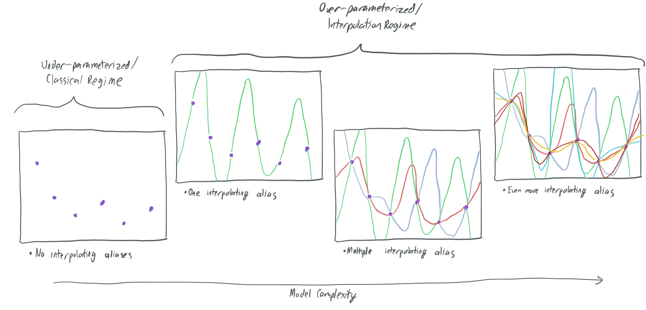
MVSS19 studies a similar setting to BLLT19 with decreasing variances. They do so by treating the over-parameterized learning model as the process of choosing between aliases—hypotheses that perfectly interpolate (or fit) the training samples and minimize empirical risk. As the complexity of a model increases beyond the point of overfitting, the number of aliases increases rapidly, which means that an empirical-risk-minimizing algorithm (like least-squares regression) has many choices of learning rules to choose from, some of which might have good generalization properties.
This paper answers two questions for a broad category of data models:
- What is the population error of the best \(d\)-parameter linear learning rule \(f: \mathbb{R}^d \to \mathbb{R}\) that interpolates all \(n\) training samples (that is, \(f(x_i) = y_i\) for all \(i \in [n]\))? They answer this question in Section 3 by characterizing the “fundamental price of interpolation.” In doing so, they show that it is essential that \(d \gg n\) for an interpolating solution to perform well. That is, dramatic over-parameterization is necessary for any learning algorithm to obtain a rule that fits the training samples and has a low expected risk.
-
When does the over-parameterized least-squares algorithm choose a good interpolating classifier? While (1) tells us that there exists some alias with low risk when \(d \gg n\), it doesn’t tell us whether this particular learning algorithm will find it. They introduce a framework in Section 4 for analyzing signal bleed (when the true signal present in the training samples is distributed among many aliases, leaving none of them with an adequate amount of signal) and signal contamination (when the noise from the training samples corrupts the chosen alias). This framework justifies the “not too fast/not too slow” conditions from BLLT19 and argues that a gradual decay of variances is necessary to ensure that least-squares obtains a learning rule that neither ignores the signal nor is corrupted by noise.
Note: The paper actually considers a general covariance matrix \(\Sigma\) for the inputs \(x_i\) and does not require that each of the \(d\) components be uncorrelated with all others. Thus, instead of considering the rate of decay of the variances of each independent component, this paper (and BLLT19) instead consider the rate of decay of the eigenvalues of \(\Sigma\). It’s then possible for favorable interpolation to occur when in cases where every component of \(x_i\) has the same variance, but the eigenvalues of \(\Sigma\) decay at a gradual rate because of correlations between components.
They have plenty of other interesting stuff too. The end of Section 4 discusses Tikhonov (ridge) regression, which adds a regularization terms and does not overfit, but does outperform least-squares interpolation for a proper choice of regularization parameters. Section 5 focuses on a broader range of interpolating regression algorithms (such as basis pursuit, which minimizes \(\ell_1\) error rather than the \(\ell_2\) error of least-squares) and proposes a hybrid method between the \(\ell_1\) and \(\ell_2\) approaches that obtains the best of both worlds. However, for the sake of simplicity, we’ll keep this summary to the two questions above.
What can go wrong with interpolation?
Towards answering these questions, the authors identify three broad cases when interpolation approaches fail.
Failure #1: Too few aliases
If \(d\) is not much larger than \(n\), then the model is over-parameterized, but only just. As a result, there are relatively few aliases that interpolate all of the samples \((x_i, y_i)\). (This roughly corresponds to the second and third panels of the above graphic.) Frequently, none of these will be any good, since they might all fall into the typical pitfalls of overfitting: in order to perfectly fit the samples, the underlying trend in the data is missed.
Noisy labels (\(y_i = \langle x_i, \beta\rangle + \epsilon_i\) for random \(\epsilon_i\) with variance \(\sigma^2\)) exacerbate these issues. If few aliases are available, most of them will be heavily affected by the noisy samples. Indeed, the authors of this paper argue that the only way to ensure the existence of an interpolating learning rule that is not knocked askew by the noise is to have many aliases. Thus, interpolation will not work without over-parameterization; we must require that \(d \gg n\). More on this later.
Failure #2: Signal bleed
In this case, we have plenty of aliases, but they’re all different:
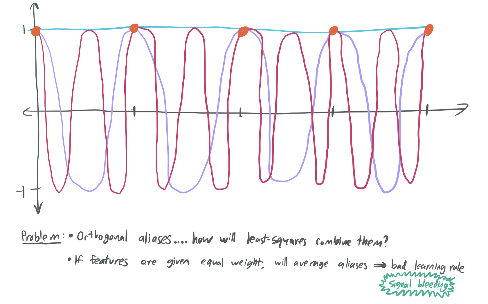
The above image shows that there are three different interpolating solutions that fit the orange points, but they are uncorrelated with one another.
(Sidebar: These aliases don’t look like linear functions, but that’s because they’re being applied to the Fourier features of the input. This will be discussed later.)
Suppose the true learning rule is represented by the cyan constant-one alias. We’re doomed if the learning algorithm chooses the purple or red aliases because those are uncorrelated with the cyan alias and will label the data with no better accuracy than chance. The least-squares algorithm will produce a learning rule that averages all three together, which will also poorly approximates the true curve. Thie phenomenon is known as signal bleed, because the helpful signal provided by the data is diluted by being distributed between several aliases that are uncorrelated.
To avoid signal bleed, the learning algorithm needs to somehow be biased in favor of lower-frequency or simpler features. This is why the BLLT19 paper requires that the variances of each component decay at a sufficiently fast rate. If they don’t, then there is no way to break ties among uncorrelated aliases, which dooms them to a bad solution.
Failure #3: Signal contamination
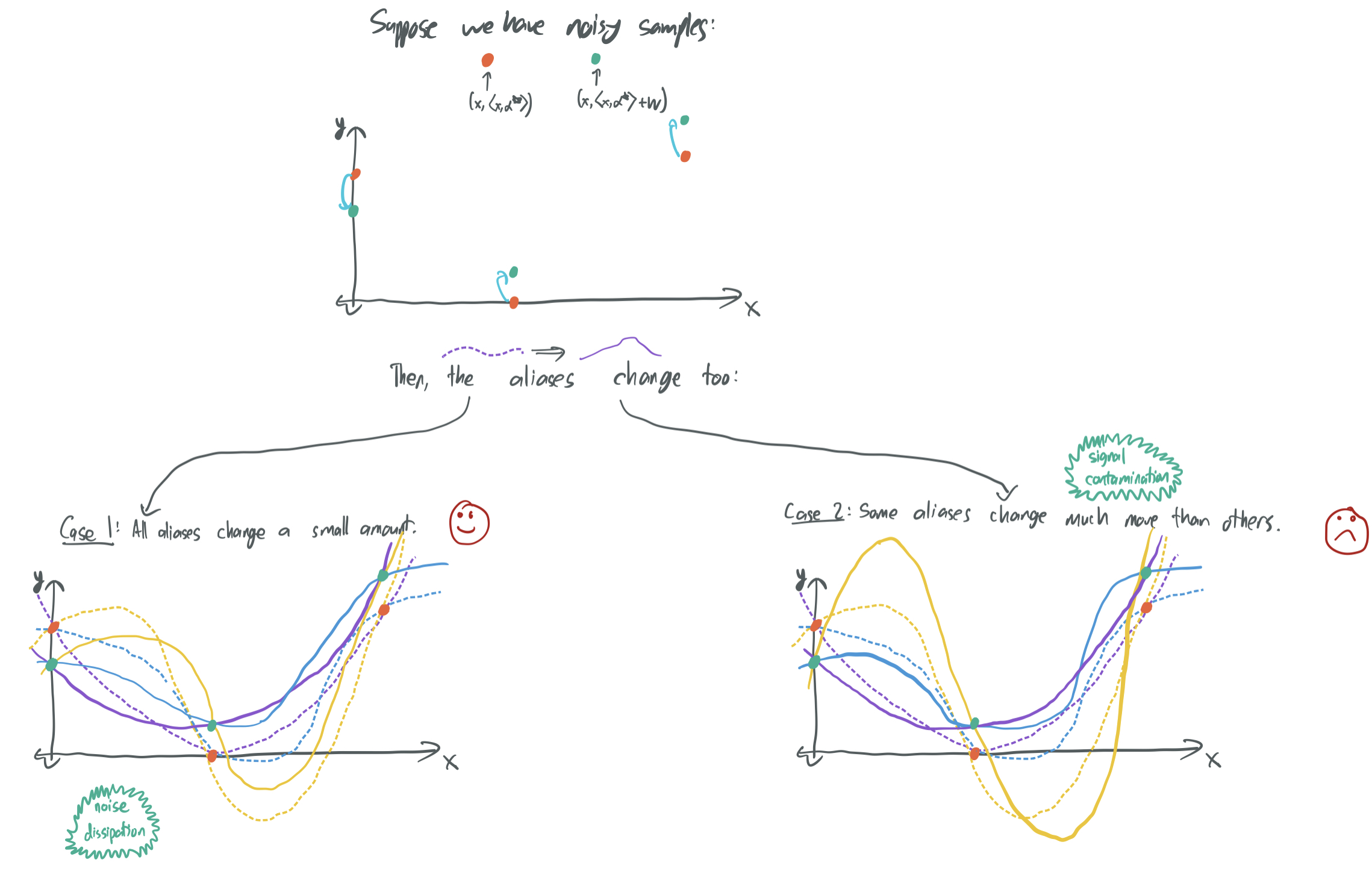
Suppose once again, we’re in a setting with many different aliases, some of which are uncorrelated with one another. If we consider the noise \(w_i\) added to each label, then every one of the aliases will somehow be corrupted when the noise is added. Ideally, we want to show that as the number of samples and number of parameters become large, the impact of the noise on the chosen interpolating alias will be minor.
For this to be possible, we have to ensure that the noise is diluted among the different aliases. This is the opposite of what we want for the signal! We know that the noise will corrupt the aliases, but if there are many uncorrelated aliases, the corruption can either be relatively evenly distributed among the different aliases (noise dissipation) or concentrated in a few (signal contamination). The first case can then be used to argue that any alias chosen by the learning algorithm will be minimally affected by noise, which is great!
One way to ensure that noise is diluted among aliases is to impose some degree of similar weight on aliases under consideration. In the land of BLLT19, this means guaranteeing that the rate of decay of variances is not too fast. This poses the trade-off explored in BLLT19 and here: There’s a sweet spot in the relative importance of different features from the perspective of the learning algorithm that must be found in order to avoid either signal bleed or signal contamination.
Before jumping in to these results more formally, we introduce two data models that we’ll refer back to.
Data models
In both cases, inputs \(x\) are chosen from some procedure and label \(y = \langle x, \beta\rangle + \epsilon\), where \(\beta\) is the unknown true signal and \(\epsilon \sim \mathcal{N}(0, \sigma^2)\) is independent Gaussian noise. We let \(X \in \mathbb{R}^{n \times d}\), \(Y \in \mathbb{R}^n\), and \(W \in \mathbb{R}^n\) contain all of the training inputs, labels, and noise respectively.
The least-squares algorithm returns the minimum-norm \(\hat{\beta} \in \mathbb{R}^d\) that interpolates the training data: \(X \hat{\beta} = Y\).
Note: This notation is slightly different than the notation used in their paper. I modified to make it line up more closely with BHX19 and BLLT19.
Model #1: Gaussian features
Every input \(x \in \mathbb{R}^d\) is drawn independenty from a multivariate Gaussian \(\mathcal{N}(0, \Sigma)\), where \(\Sigma \in \mathbb{R}^{d\times d}\) is a covariance matrix.
Model #2: Fourier features
For any \(j \in [d]\), we define the \(j\)th Fourier feature to be a function \(\phi_j: [0, 1] \to \mathbb{C}\) with \(\phi_j(t) = e^{2p (j-1) i t}\). Because \(e^{iz} = \cos(z) + i \sin(z)\), \(\phi_j(t)\) can be thought of as a sinusoidal function with frequency increasing with \(j\). For any \(t \in [0, 1]\), it’s Fourier features are \(\phi(t) = (\phi_1(t), \dots, \phi_d(t)) \in \mathbb{C}^d\).
Notably, these features are orthonormal and uncorrelated. That is,
\[\langle \phi_j, \phi_k \rangle = \mathbb{E}_{t \sim \text{Unif}[0, 1]}[\phi_j(x) \phi_k(x)] = \begin{cases} 1 & \text{if } j=k, \\ 0 & \text{otherwise.} \end{cases}\]To learn more about orthonormality and why its a desirable trait in vectors and functions, check out my post on the subject.
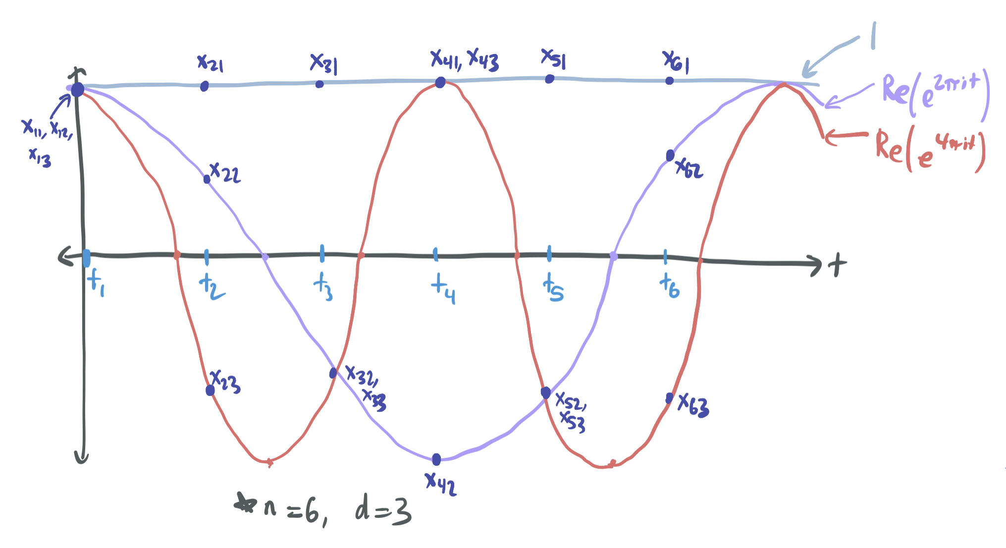
We generate the training samples by choosing \(n\) evenly spaced points on the interval \([0, 1]\): \(t_j = \frac{i-1}{n}\) for all \(i \in [n]\). The features of the \(j\)th sample are \(x_j = \phi(t_j) = (1, e^{2 \pi i t_j}, e^{2\pi(2i) t_j}, \dots, e^{2\pi((d-1)i) t_j}) \in \mathbb{C}^d\). The feature vectors for each sample are also orthonormal: \(\langle x_j, x_k \rangle = 1\) if \(j = k\) and \(0\) otherwise.
The below image gives a visual of the sinusoidal interpretation of Fourier features and the training samples:
The necessity of over-parameterization
Section 3 of the paper studies the “fundamental price of interpolation” by asking about how good the best interpolating classifier can be. Specifically, the ideal test risk of any interpolating classifier:
\[\mathcal{E}^* = \min_{\beta \in \mathbb{R}^d: X \beta = Y} \mathbb{E}_{(x, y)}[(y - \langle x, \beta\rangle)^2] - \sigma^2.\]The condition \(X \beta = Y\) ensures that \(\beta\) does indeed fit all of the training samples. The variance of the noise \(\sigma^2\) is subtracted because no classifier can ever hope to have risk better than the noise, since every label will be corrupted.
They prove upper- and lower-bounds on \(\mathcal{E}^*\) that hold with high probability. In particular, by Corollaries 1 and 2, with probability 0.9:
- Under the Gaussian features model, \(\mathcal{E}^* = \Theta(\frac{\sigma^2 n}{d})\).
- Under the Fourier features model, \(\mathcal{E}^* = \Omega(\frac{\sigma^2 n}{d \log n})\).
Therefore, in order to guarantee that the risk approaches the best possible as \(n\) and \(d\) grow, it must be the case that \(d \gg \sigma^2 n\). That is, it’s essential for the model to be over-parameterized for the interpolation to be favorable. This formalizes Failure #1 by highlighting that without enough aliases (which are provided by having a highly over-parameterized model), even the best alias will have poor performance.
These proofs first use linear algebra to exactly represent \(\mathcal{E}^*\) in terms of inputs \(X\), covariance \(\Sigma\), and noise \(\epsilon\). Then, they apply concentration bounds to show that the risk is close to its expectation with high probability over the input data and the noise.
Not too fast; not too slow
Here, we recap Section 4 of the paper while studying the Fourier features setting. In doing so, we explain how Failures #2 and #3 can occur. We focus on Fourier features because their orthogonality properties make the concepts of signal bleed and signal contamination much cleaner.
Signal bleed
Consider a simple learning problem where each \(x\) is a Fourier feature and \(y = 1\) no matter what. (There is no noise here.) In this case, our samples will be of the form \((\phi(t_1), 1), \dots, (\phi(t_n), 1)\) for \(t_1, \dots, t_n\) evenly spaced in \([0, 1]\).
First, we ask ourselves which solutions will interpolate between the samples. Since the \(j\)th Fourier feature is the function \(\phi_j(t) = e^{2p (j-1) i t}\), the first Fourier feature \(\phi_1(t) = 1\) is an interpolating alias. (It’s also the correct alias.) However, so too will be \(\phi_j\) when \(j-1\) is a multiple of \(n\). This is orthogonal (uncorrlated) to the first feature (and all other Fourier features). If there are \(d\) Fourier features and \(n\) samples for \(d \gg n\), there are \(\frac{d}{n}\) interpolating aliases, all of which are orthogonal.
This is a problem. This forces our algorithm to choose between \(\frac{d}{n}\) different candidate learning rules, all of the which are completely uncorrelated with one another, without having any additional information about which one is best. Indeed, the interpolating learning rule can be any function of the form \(\sum_{j = 0}^{d/n} a_j \phi_{nj+1}(t)\) for \(\sum_{j = 0}^{d/n} a_j = 1\).
How does the least-squares algorithm choose a parameter vector \(\beta\) from all of these interpolating solutions? It chooses the one with the smallest \(\ell_2\) norm. By properties of orthogonality, this is equivalent to choosing the function minimizing \(\sum_{j = 0}^{d/n} a_j^2\), which is satisfied by taking \(a_j = \sqrt{\frac{n}{d}}\). This means that \(\beta_1 = \sqrt{\frac{n}{d}}\). Equivalently, the true feature \(\phi_1\) contributes only a \(\sqrt{\frac{n}{d}}\) amount of influence on the learning rule, which diminishes as \(d\) grows and the model becomes further over-parameterized.
This is why we refer to this failure mode (Failure #2) as signal bleed: the signal conveyed in \(\phi_1\) bleeds into all other \(\phi_{jn + 1}\) until the true signal has almost no bearing on the outcome.
How can this be fixed? By giving a higher weight to “simpler” features in order to indicate some kind of preference for these features. The higher weight permits the \(\ell_2\) norm of a classifier to contain a large amount of influence \(\phi_1\) without incurring a high cost.
To make this concrete, let’s rescale each \(\phi_j\) such that \(\phi_j = \sqrt{\lambda_j} e^{2p (j-1) i t}\). Now, the interpolating aliases are \(\frac{1}{\sqrt{\lambda_j}} \phi_j\) whenever \(j\) is one more than a multiple of \(n\), which means that the higher-frequency features will be more costly to employ. This time, we can express any learning rule in the form \(\sum_{j = 0}^{d/n} \frac{a_j}{\sqrt{\lambda_j}} \phi_{nj+1}(t)\) for \(\sum_{j = 0}^{d/n} a_j = 1\). Least-squares will then choose the learning rule whose \(a_j\) values minimize \(\sum_{j = 0}^{d/n} \frac{a_j^2}{\lambda_j}\). This will be done by taking:
\[a_j = \frac{\lambda_j}{\sum_{k=0}^{d/n} \lambda_{kn +1}},\]Going back to our Fourier setting where \(\phi_1\) is the only true signal, our classifier will perform best if \(a_1 \approx 1\), which occurs if \(\frac{\lambda_0}{\sum_{k=0}^{d/n} \lambda_{kn +1}} \to 1\) as \(n\) and \(d\) become large. (The quantity that must approach 1 is known as the survival factor in this paper.) For this to be possible, there must be a rapid drop-off in \(\lambda_j\) as \(j\) grows.
Interestingly, this coincides with BLLT19’s requirements for “benign overfitting.” The survival factor coincides is the inverse of their \(r_0(\Sigma)\) term, which captures the gap between the largest variance and the sum of the other variances. As was discussed in that blog post, the quantity must be much smaller than \(n\) for their bound to be non-trivial.
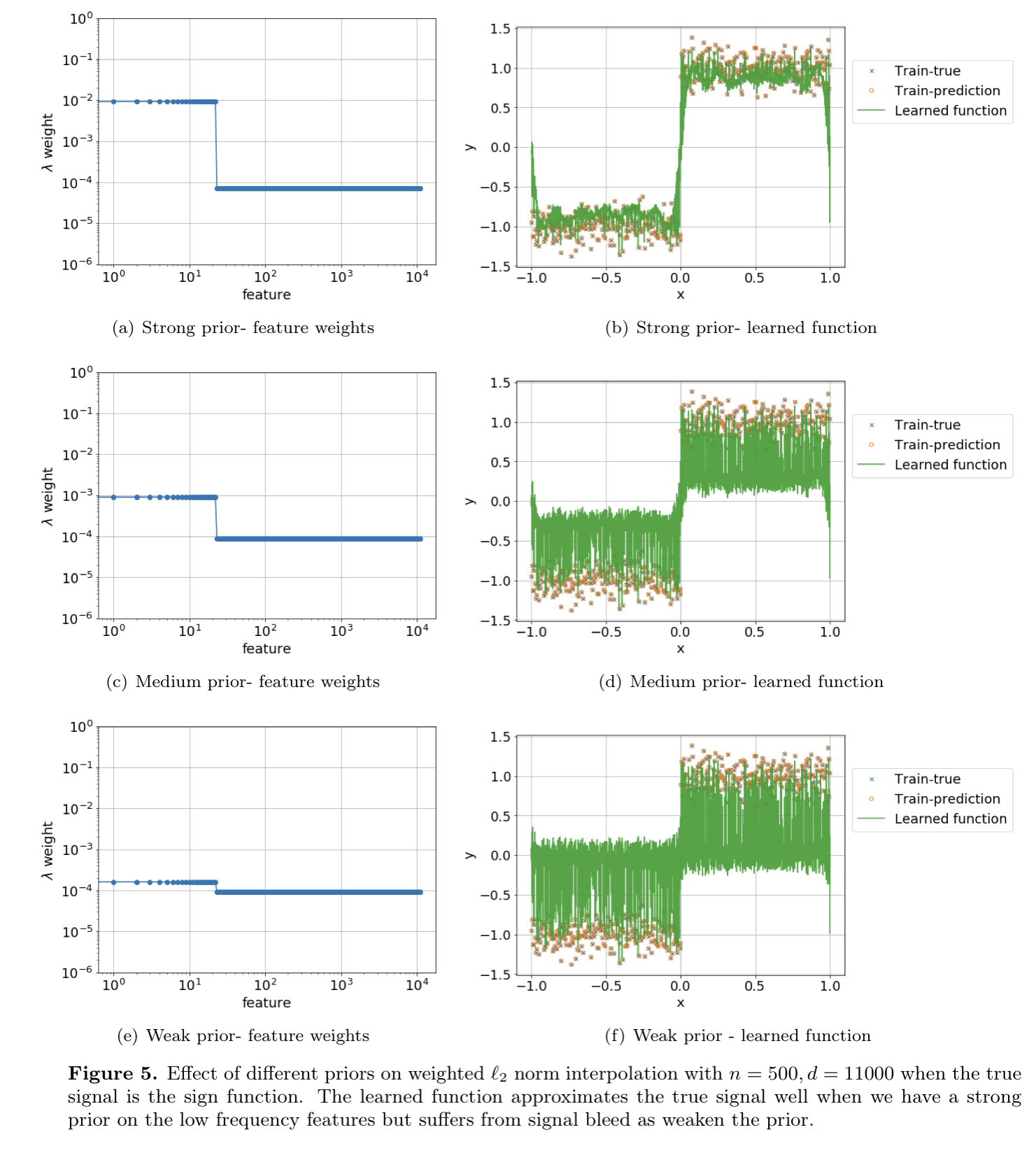
Figure 5 of their paper provides a nice visualization of how dropping the weights on high-frequency can lead to better interpolating solutions that avoid signal bleed. The top plot has a large gap between the weights on the low-frequency features and the high-frequency features, which prevents least-squares from giving too much preference to the high-frequency features that just happen to interpolate the training data. The bottom plot produces a spiky and inconsistent plot because it fails to do so.
This logic seems circular somehow: in order to have good interpolation, we must be able to select for the good features and weight them strongly enough so that their aliases override orthogonal aliases. However, if we know the good features, why include the bad features in the first place? The next section part discusses why it’s important in the interpolation regime to not let the importance of features (represented by \(\lambda_j\)) drop too rapidly.
Signal contamination
In the previous section, we were concerned about the “true signal” of \(\phi_1\) being diluted by the preference of least-squares for higher-frequency Fourier features. To combat that, it was necessary to drop the variances of the high-frequency features by some sequence \(\lambda_j\) that decreases sufficiently quickly.
Here, we’re concerned with the opposite issue: the incorrect influence of orthonormal high-frequency aliases and noise on the learning rule inferred by least-squares. In this Fourier features setting, all contributions from other aliases will necessarily increase the risk because the other aliases are all orthogonal to the signal \(\phi_1\). As before, we can quantify the minimum error caused by the inclusion of other aliases in the prediction, which we’ll call the contamination:
\[C = \sqrt{\sum_{k = 1}^{d/n} \hat{\beta}_{kn + 1}^2}.\]In the case of least-squares regression, we have:
\[C = \frac{\sqrt{\sum_{k=1}^{d/n} \lambda_{kn+1}}}{\sum_{k = 0}^{d/n} \lambda_{kn +1}}.\]We’re interested in finding weights \(\lambda_j\), which ensure that the contamination \(C\) becomes very small a regime where \(d\) and \(n\) are very large. One way to do so is to choose \(\lambda_j\) such that \(\sqrt{\sum_{k=1}^{d/n} \lambda_{kn+1}} \ll\sum_{k = 1}^{d/n} \lambda_{kn +1}\), which occurs when the sum of weights is large and the decay of \(\lambda\) is heavy-tailed. That is, to avoid having spurious features have a lot of bearing on the final learning rule, one can require that \(\lambda\) decays very slowly, so that the lower-frequency spurious features are not given much more weight than the higher-frequency features.
Taken together, this section and the previous section impose a trade-off how features should be weighted.
- To avoid signal bleeding, it’s necessary for a relatively small number of features to have much more weight than the rest of them.
- To avoid signal contamination, the remaining features need to jointly have a large amount of weight and the weights cannot decay too quickly.
This is the same trade-off presented by BLLT19 with their \(r_k(\Sigma)\) and \(R_k(\Sigma)\) terms. For their bounds to be effective, it’s necessary to have that \(r_0(\Sigma) \ll n\) (prevent signal bleed by mandating decay of feature variances) and \(R_{k^*}(\Sigma) \gg n\) where \(k^*\) is a parameter that divides high-variance and low-variance features (prevent signal contamination by requiring that the variances decay sufficiently slowly).
Conclusion and next steps
Like the other papers discussed so far, the results of this paper apply to a very clean setting. The Fourier features examples illustrate these contamination-vs-bleed trade-offs in a very clean way because the orthogonality of the features means that all features other than the signal are strictly detrimental. Still, this paper is nice because it motivates the mathematical conditions specified in BLLT19 and gives more intuition into when one should expect least-squares interpolation to succeed.
The paper suggests that further works focus on the powers of approximation of more complex models and how they relate to success in the interpolation regime. This is where there’s a key difference between BHX19 and BLLT19/MVSS19. The over-parameterized models in the former explicitly have more information in comparison to their under-parameterized counterparts, so they have a clear advantage in the kinds of functions they can approximate. On the other hand, the success of over-parameterized models in BLLT19 and MVSS19 are solely dependent on the relative variances of many features; they don’t say anything about the fact that most over-parameterized models can express more kinds of functions. The authors hope that future work continues to study interpolation through the lens of signal bleed and signal contamination, but that they also find a way to work in the real approximation theoretic advantages that over-parameterized models maintain over other models.
I personally enjoyed reading this paper a lot, because I found it very intuitive and well-written. I’d recommend checking it out directly if you find this interesting!
Comments