[OPML#5] BL20: Failures of model-dependent generalization bounds for least-norm interpolation
[candidacy technical learning-theory over-parameterized least-squares This is the fifth of a sequence of blog posts that summarize papers about over-parameterized ML models.
I really enjoyed reading this paper, “Failures of model-dependent generalization bounds for least-norm interpolation,” by Bartlett and Long. (The names are familiar from BLLT19.) It follows in the vein of papers like ZBHRV17 and NK19, which demonstrate the limitations of classical generalization bounds.
This work differs from the double-descent papers that have been previously reviewed on this blog, like BHX19 [OPML#1], BLLT19 [OPML#2], MVSS19 [OPML#3], and HMRT19 [OPML#4]. These papers argue that there exist better bounds on generalization error for over-parameterized linear regression than the ones typically suggested by classical approaches like VC-dimension and Rademacher complexity. However, they dont prove that there cannot be better “classical” generalization bounds; they just show that the well-known bounds are inferior to their proposed bounds. On the other hand, this paper proves that a broad family of traditional generalization bounds are unable to explain the phenomenon of the success of interpolating methods.
The gist of the argument is that it’s not sufficient to look at the number of samples and the complexity of the hypothesis to explain the success of interpolating models. Successful bounds must take into account more information about the data distribution. Notably, the bounds in BHX19, BLLT19, MVSS19, and HMRT19 all rely on properties of the data distribution, like the eigenvalues of the covariance matrix and the amount of additive noise in each label. The current paper (BL20) posits that such tight bounds are impossible without access to this kind of information.
In this post, I present the main theorem and give a very hazy idea about why it works. Let’s first make the learning problem precise.
Learning problem
- We have labeled data \((x, y) \in \mathbb{R}^d \times \mathbb{R}\) drawn from some distribution \(P\).
- They restrict \(P\) to give it nice mathematical properties. Specifically, the inputs \(x \in \mathbb{R}^d\) must be drawn from a Gaussian distribution and \((x, y)\) must have subgaussian tails. We’ll call these “nice” distributions.
- Let the risk of some prediction rule \(h: \mathbb{R}^d \to \mathbb{R}\) be \(R_P(h) = \mathbb{E}_{x, y}[(y - h(x))^2]\).
- Let \(R_P^*\) be the best risk over all \(h\).
- The goal is to consider bounds on \(R_P(h) - R_P^*\), where \(h\) is an least-norm interpolating learning rule on \(n\) training samples.
- i.e. \(h(x) = \langle x, \theta\rangle\) where \(\theta \in \mathbb{R}^d\) minimizes the least-squares error: \(\sum_{i=1}^n(\langle x_i, \theta\rangle - y_i)^2\). Ties are broken by choosing the \(\theta\) that minimizes \(\|\theta\|_2\). The interpolation regime occurs when the least-squares error is zero.
- We consider bounds \(\epsilon(h, n, \delta)\), such that \(R_p(h)- R_P^{*} \leq \epsilon(h, n, \delta)\) with probability \(1 - \delta\) over the \(n\) training samples from \(P\), for which \(h\) is least-norm interpolating.
- Notably, these bounds cannot include any more information about the learning problem; these must hold for any distribution \(P\).
- For the theorem to work, they restrict themselves to bounds that are bounded antimonotonic, which means that they cannot suddenly become much worse as the number of samples increases. (e.g. \(\epsilon(h, 2n, \delta)\) cannot be much larger than \(\epsilon(h, n, \delta)\).)
The result
Now, I give a rather hand-wavy paraphrase of the theorem:
Theorem 1: Suppose \(\epsilon\) is a bound that depends on \(h\), \(n\), and \(\delta\) that applies to all nice distributions \(P\). Then, for a “very large fraction” of values of \(n\) as \(n\) grows, there exists a distribution \(P_n\) such that
\[\mathrm{Pr}_{P_n}[R_{P_n}(h) - R_{P_n}^* \leq O(1 / \sqrt{n})] \geq 1 - \delta\]but
\[\mathrm{Pr}_{P_n}[\epsilon(h, n, \delta) \geq \Omega(1)] \geq \frac{1}{2},\]where \(h\) is the least-norm interpolant of a set of \(n\) points drawn from \(P_n\). The probabilities above refer to randomness from the training sample drawn from \(P_n\).
Let’s break this down and talk about what it means.
The generalization bound \(\epsilon\) can depend on the minimum-norm interpolating prediction rule \(h\), the number of samples \(n\), and the confidence parameter \(\delta\). It cannot depend on the distribution over samples \(P\), and it must apply to all such “nice” distributions. This opens up the possibility that a satisfactory bound \(\epsilon\) could perform much better on some distributions than others.
-
This result particularly applies to generalization bounds that make use of some property of the prediction rule \(h\). For instance, it demonstrates the limitations of this 1998 Bartlett paper, which gives generalization bounds that are small when the parameters of \(h\) have small norms.
-
Note that this isn’t really talking about “traditional” capacity-based generalization bounds, like those that rely on VC-dimension. These capacity-based bounds are applied to the hypothesis class \(\mathcal{H}\) that contains \(h\), rather than the prediction rule \(h\) itself.
These kinds of bounds are already overly pessimistic in the over-parameterized regime, however. Measurements of the capacity of \(\mathcal{H}\)—like the VC-dimension and the Rademacher complexity—will always lead to vacuous generalization bounds for interpolating classifiers because those bounds rely on limiting the expressive power of hypotheses in \(\mathcal{H}\). From the lens of capacity-based generalization approaches, overfitting is always bad, which makes a nontrivial analysis of interpolation methods impossible with these tools.
\(\epsilon\) does indeed perform much better on some distributions than others. The meat and potatoes of the proof shows the existence of some nice distribution where a bound \(\epsilon\) necessarily underperforms, even though the minimum-norm interpolating solution actually has a small generalization error.
-
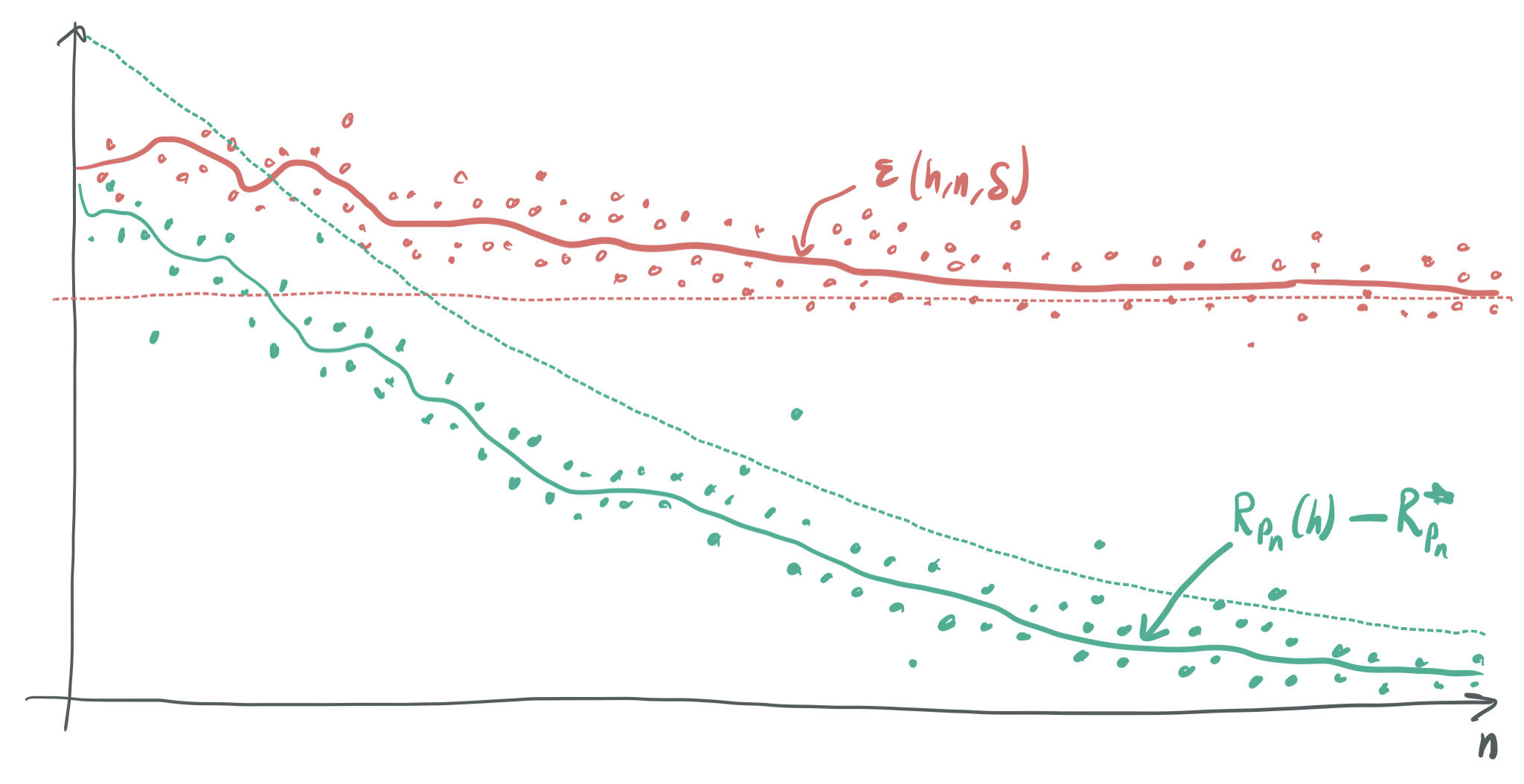
The first inequality in the theorem demonstrates how the minimum-norm interpolating classifier does well. This is represnted by the the true generalization errors lying below the green dashed line, which corresponds to the bound in the first inequality. As \(n\) grows, the true generalization error approaches zero with high probability.
-
On the other hand, the underperformance is illustrated by the second inequality, which shows that the bound \(\epsilon\) often cannot guarrantee that the generalization error is smaller than some constant as \(n\) becomes large. As visualized above, the bound \(\epsilon\) (represented by red dots with a red line corresponding to the expected value of \(\epsilon\)) will most of the time (but not always) lie above the constant curve denoted by the dashed red line. This isn’t great, because we should expect an abundance of training samples \(n\) to translate to an error bound that approaches zero as \(n\) approaches infinity.
So far, nothing has been said about the dimension of the inputs, \(d\). The authors define \(d\) within the context of the distributions \(P_n\) as roughly \(n^2\). Thus, \(d \gg n\) and this problem deals squarely with the over-parameterized regime.
To reiterate, the key takeaway here is that the data distribution is very important for evaluating whether successful generalization occurs. Without knowledge of the data distribution, it’s impossible to give accurate generalization bounds for the over-parameterized case (\(d \gg n\)).
Proof ideas
The main strategy in this proof is to show the existence of a “good distribution” \(P_n\) and a “bad distribution” \(Q_n\) that are very similar, but where minimum-norm interpolation yields a much smaller generalzation error on \(P_n\) than \(Q_n\). This gap forces any valid generalization error bound \(\epsilon\) to be large, despite the fact that the the minimum-norm interpolator has small generalzation error for \(P_n\).
To satisfy the similarity requirement, \(P_n\) and \(Q_n\) must be indistinguishable with respect to \(h\). Consider full training samples of \(n\) \(d\)-dimensional inputs and labels \((X_P, Y_P), (X_Q, Y_Q) \in \mathbb{R}^{n \times d} \times \mathbb{R}^n\) drawn from the two respective distributions. Then, the probability that \(h\) is the minimum-norm interpolator of \((X_P, Y_P)\) must be identical to the probability that it is the minimum-norm interpolator of \((X_Q, Y_Q)\). If this is the case, then \(\epsilon\) must be defined to ensure that each of
\[\epsilon(h, n, \delta) \geq R_{P_n}(h) - R_{P_n}^* \quad \text{and} \quad \epsilon(h, n, \delta)\geq R_{Q_n}(h) - R_{Q_n}^*\]hold with probability \(1 - \delta\). This then means that it must be the case that for any \(t \in \mathbb{R}\):
\[\mathrm{Pr}_{P_n}[\epsilon(h, n, \delta) \geq t] \geq \max(\mathrm{Pr}_{P_n}[R_{P_n}(h) - R_{P_n}^* \geq t], \mathrm{Pr}_{Q_n}[R_{Q_n}(h) - R_{Q_n}^* \geq t]).\]To prove the theorem, it suffices to show \(R_{P_n}(h) - R_{P_n}^*\) is very small and \(R_{Q_n}(h) - R_{Q_n}^*\) is large with high probability. This forces \(\epsilon(h, n, \delta)\) to be large and \(R_{P_n}(h) - R_{P_n}^*\) to be small with high probability, which concludes the proof.
A key idea towards showing this gap between the generalization of \(P_n\) and \(Q_n\) is to define distributions that behave very differently in testing, despite being indistinguishable from the standpoint of training. To implement this idea, \(Q_n\) will reuse samples in testing phase, while \(P_n\) will not.
Now, we define the two distributions, with the help of a third “helper” distribution \(D_n\).
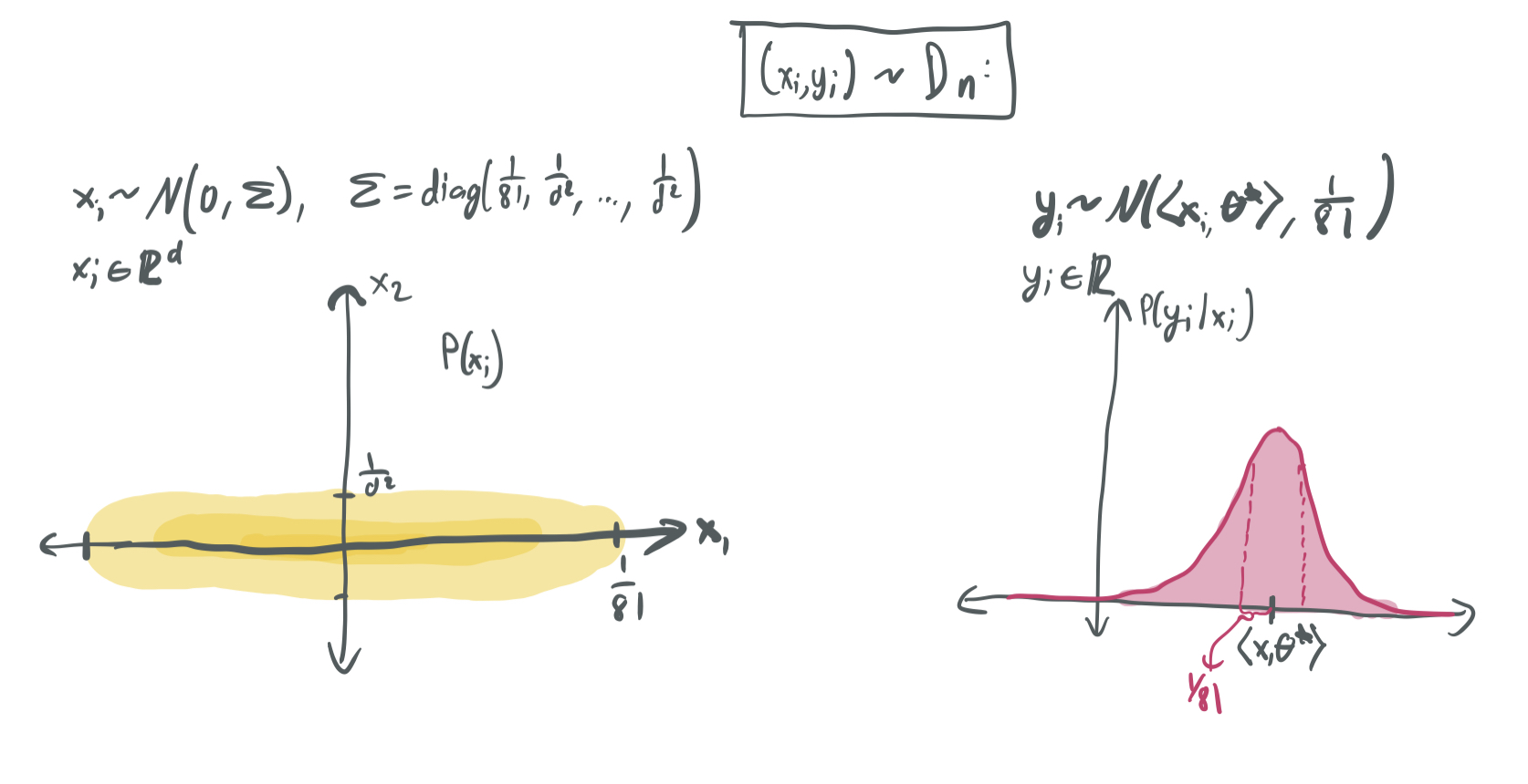
\(D_n\): The skewed Gaussian distribution
We draw an input \(x_i\) from the \(d\)-dimensional Gaussian distribution \(\mathcal{N}(0, \Sigma)\) with mean zero and diagonal covariance matrix \(\Sigma\) with
\[\Sigma_{j,j} = \lambda_j = \begin{cases} \frac{1}{81} & j = 1 \\ \frac{1}{d^2} & j > 1. \end{cases}\]When \(d\) is large, this corresponds to a distribution where \(x_1\) will be very large relative to \(x_2, \dots, x_d\), which trend towards zero. The label \(y_i\) is drawn by taking \(y_i = \langle x_i, \theta\rangle + \epsilon_i\), where \(\epsilon_i \sim \mathcal{N}(0, \frac{1}{81})\). Thus, the noise is drawn at the scale of the dominant first coordinate.
We use this skewed distribution because it works beautifully with the bounds in the minimum-norm interpolant that are laid out in BLLT19. Using notation from my blog post on BLLT19, we can characterize the effective dimensions \(r_k(\Sigma)\) and \(R_k(\Sigma)\), which yield clean risk bounds.
\[r_k(\Sigma) = \frac{\sum_{j > k} \lambda_j}{\lambda_{k+1}} = \begin{cases} \frac{\frac{1}{81} + \frac{d-1}{d^2}}{\frac{1}{81}} = \Theta(1) & k = 0 \\ \frac{\frac{d-k}{d^2}}{\frac{1}{d^2}} = d-k & k > 0. \end{cases}\] \[R_k(\Sigma) = \frac{\left(\sum_{j > k} \lambda_j\right)^2}{\sum_{j > k} \lambda_j^2} = \begin{cases} \frac{\left(\frac{1}{81} + \frac{d-1}{d^2}\right)^2}{\frac{1}{81^2} + \frac{d-1}{d^4}} = \Theta(1) & k = 0 \\ \frac{\left(\frac{d-k}{d^2}\right)^2}{\frac{d-k}{d^4}} = d-k & k > 0. \end{cases}\]By taking \(k^* = 1\) and applying the bound, then with high probability:
\[R(\hat{\theta}) = O\left(\|\theta^*\|^2 \lambda_1\left( \sqrt{\frac{r_0(\Sigma)}{n}} + \frac{r_0(\Sigma)}{n}\right) + \sigma^2\left(\frac{k^*}{n} + \frac{n}{R_{k^*}(\Sigma)}\right) \right)\] \[= O\left(\|\theta^*\|^2\left(\frac{1}{\sqrt{n}} + \frac{1}{n}\right) + \frac{1}{81}\left(\frac{1}{n} + \frac{n}{d-1}\right)\right).\]If we take \(d = n^2\), then this term trends towards zero at a rate of \(\frac{1}{\sqrt{n}}\) as \(n\) approaches infinity, which validates the kind of bound w’ere looking at for \(P_n\). (Note: \(d\) does not exactly equal \(n^2\) in the paper; there are a few more technicalities here that we’re glossing over.)
This gives us an example where minimum-norm interpolation does fantastically. However, it does not show why the generalization bound \(\epsilon(h, n, \delta)\) cannot be tight. To do so, we define the actual two distributions we care about—\(Q_n\) and \(P_n\)—in terms of \(D_n\).
\(Q_n\): Poor interpolation from sample reuse
The first confusing thing about \(Q_n\) is that it’s a random distribution. That is, we can think of \(Q_n\) being drawn from a distribution over distributions \(\mathcal{Q}_n\), since it depends on a random sample from \(D_n\).
To define \(Q_n\), draw \(m = \Theta(n)\) independent samples \((x_i, y_i)_{i \in [m]}\) from \(D_n\). \(Q_n\) will be supported on these \(m\) samples.
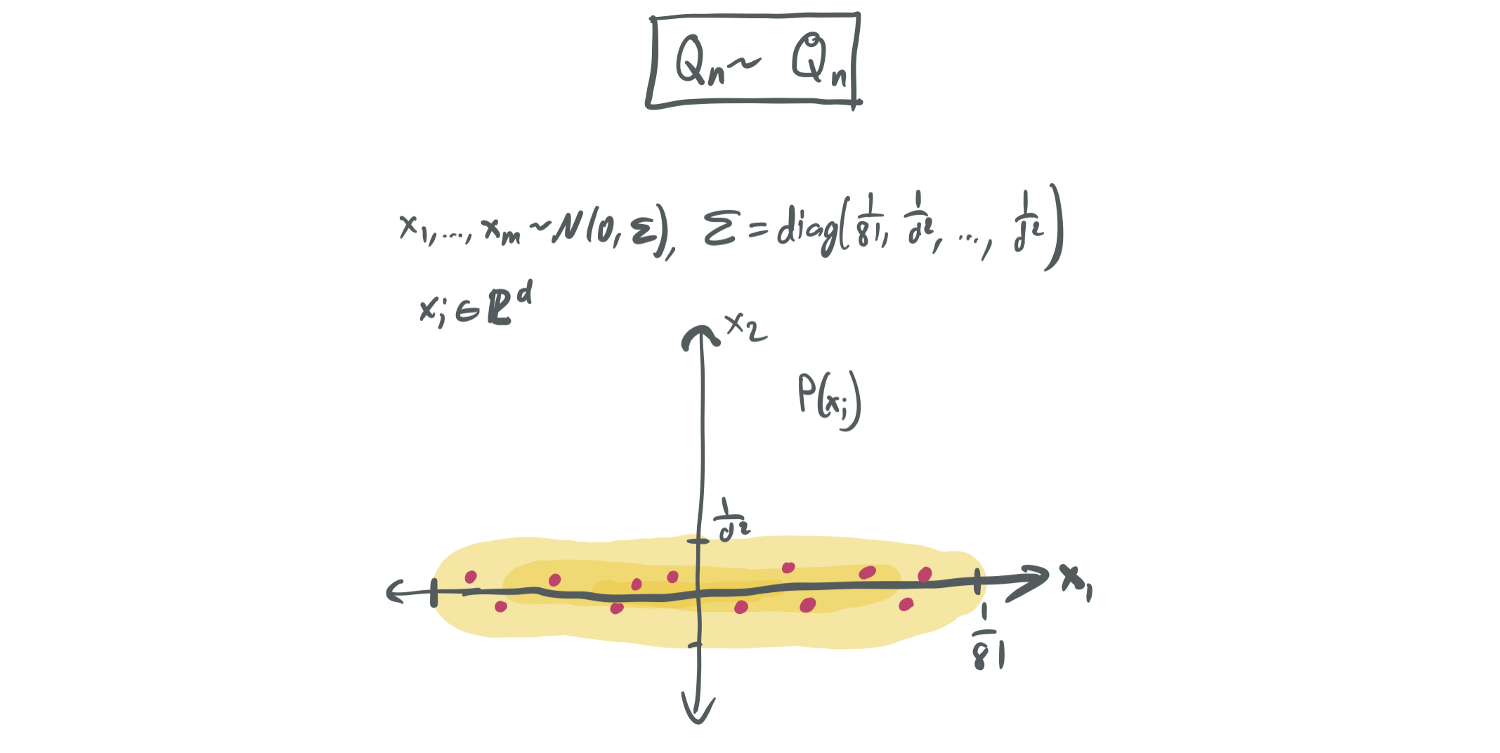
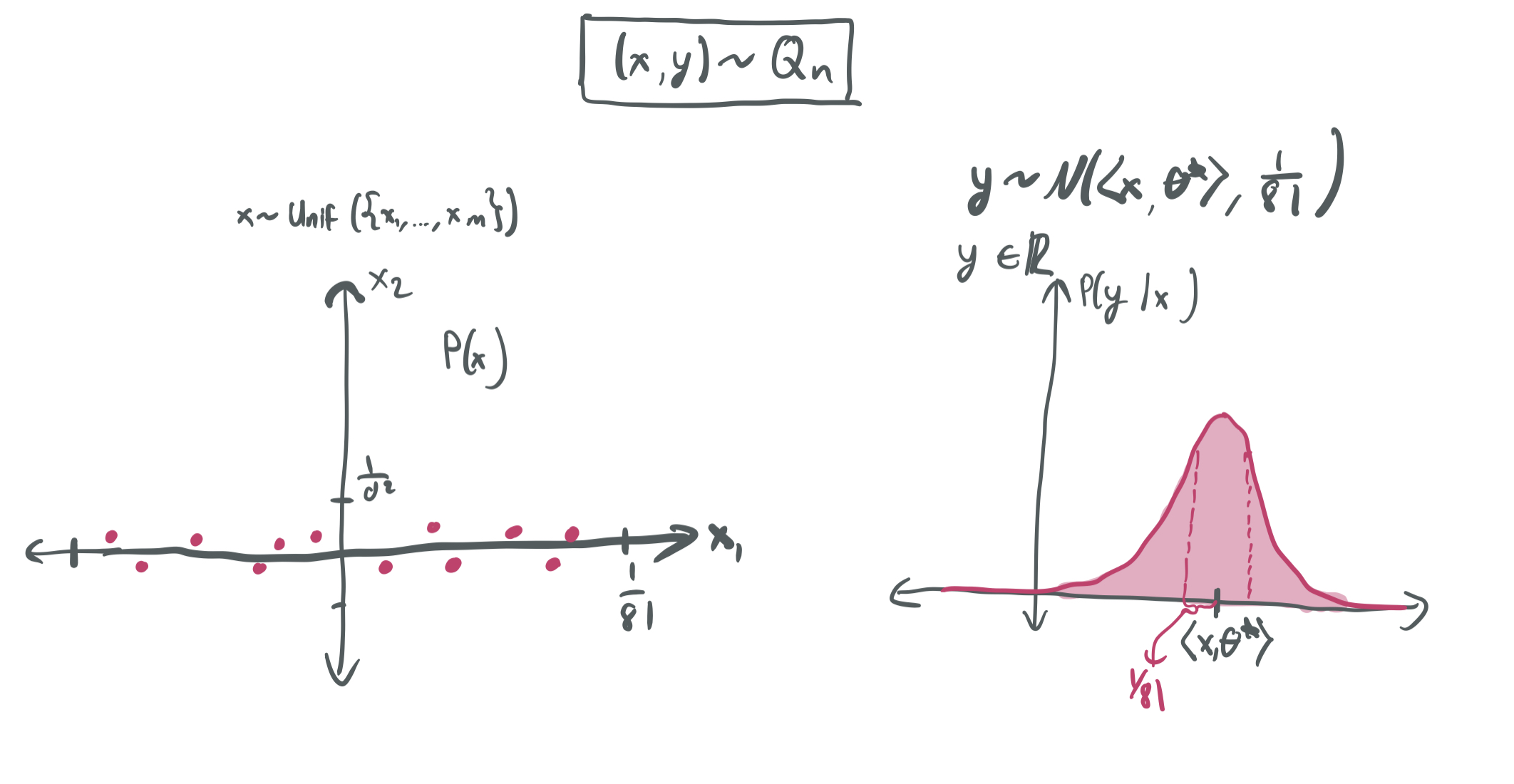
After fixing these samples, we can draw \((x, y)\) from \(Q_n\) by first uniformly selecting \(x\) from \(\{x_1, \dots, x_m\}\), the set of pre-selected points. Then, we choose \(y\) using the same approach that we did for \(D_n\): \(y = \langle x, \theta\rangle + \epsilon\) for \(\epsilon \sim \mathcal{N}(0, \frac{1}{81})\).
What this means is that the training inputs \(x_i\) for \(i \in [n]\) will exactly reoccur in the expected risk, albeit with different labels \(y_i\). This differs greatly from \(D_n\), where the continuity of the distribution over \(x_i\)’s ensures that the same exact sample would never realistically be chosen in “testing.”
The crux of the argument that \(Q_n\) is “bad” comes from Lemma 5, which suggests that least-norm interpolation will perform poorly on inputs \(x_i\) that show up exactly once in the training set. When these are drawn again when computing the expected risk (with new labels), they’ll have substantially higher error than would a random input from \(D_n\). This allows the authors to show that—for a proper choice of \(m\)—
\[\mathrm{Pr}_{Q_n}[R_{Q_n}(h) - R_{Q_n}^* \geq \Omega(1)] \geq \frac{1}{2}.\]Now, it only remains to show that \(Q_n\) is indistinguishable in the training phase from a “good” distribution that has low risk for least-norm interpolation.
\(D_n\) is good, but \(Q_n\) unfortunately cannot be contrasted to \(D_n\) in this manner. Because \(D_n\) never repeats training samples, the two have somewhat different distributions over interpolators \(h\). Instead, we define \(P_n\) in a slightly different way to have the nice interpolation properties of \(D_n\), while being identical to \(Q_n\) in the training phase.
\(P_n\): \(D_n\) but with extra samples
The idea with \(D_n\) is that it draws inputs \(x_i\) from \(P_n\), but that it will occasionally draw more than one and average their labels \(y_i\) together to produce a new label.
This provides indistinguishability from \(Q_n\) in the training phase. Both draw a collection of samples—with some of them appearing multiple times in the training set—and both minimum-norm interpolators will take these properties into account. This indistinguishability is proved in Lemma 7 and relies on careful choices of the number of original samples \(m\) for \(Q_n\) and the amount of repeated samples in \(P_n\). This idea is put together with Lemma 5 (which shows that \(Q_n\) has poor minimum-norm interpolation behavior) to show that \(\epsilon(h, n, \delta)\) cannot be small.
However, \(P_n\) is not a random distribution and it will not carry that repetition over to the “evaluation phase.” The distribution used to evaluate risk—like \(D_n\) and unlike \(Q_n\)—will not contain any of the same \(x_i\)’s that were used in the training phase. This causes the interpolation guarantees to be roughly the same as \(D_n\). This gives the gap we’re looking for, which is formalized in Lemma 10.
Put together with Lemma 5, this gives the bound we’re looking for and concludes the story that the success (or lack thereof) of minimum-norm interpolation can only be understood by considering the data distribution, and not just the number of samples \(n\) and properties of the interpolants \(h\).
Thanks for reading the post! As always, I’d love to hear any thoughts and feedback. Writing these is very instructive for me to make sure I actually understand the ideas in these papers, and I hope they provide some value to you too.
Comments