[OPML#10] MNSBHS20: Classification vs regression in overparameterized regimes: Does the loss function matter?
[candidacy technical learning-theory over-parameterized This is the tenth of a sequence of blog posts that summarize papers about over-parameterized ML models, which I’m writing to prepare for my candidacy exam. Check out this post to get an overview of the topic and a list of what I’m reading.
Once again, we discuss a paper that shows how hard-margin support vector machines (SVMs) (or maximum-margin linear classifiers) can experience benign overfitting when the learning problem is over-parameterized. The paper, “Classification vs regression in overparameterized regimes: Does the loss function matter?”, was written by a Vidya Muthukumar, Adhyyan Narang, Vignesh Subramanian, Mikhail Belkin, Daniel Hsu (my advisor!), and Anant Sahai.
While the kinds of results are similar to the ones discussed in last week’s post, the methodology is quite different. Rather than studying the properties of the iterates of gradient descent, this paper shows that minimum-norm linear regression and SVMs coincide in the over-parameterized regime and shows that the models behave similarly in those cases; this phenomenon is known as support vector proliferation and discussed in depth by a follow-up paper by Daniel, Vidya, and Ji (Mark) Xu and by my NeurIPS paper with Navid Ardeshir and Daniel.
To make the point, the paper considers a narrow regime of data distributions and categorizes those distributions to determine (1) when the outputs of OLS regression and SVM classification coincide and (2) when each of those have favorable generalization error as the number of samples \(n\) and dimension \(d\) trend towards infinity. We introduce their bilevel ensemble input distribution and their 1-sparse linear model for determining labels. Their results show that under similar conditions to those explored in BLLT19, benign overfitting is possible for classification algorithms like SVMs. Indeed, for their distributional assumptions, benign overfitting is more common for classification than regression.
OLS and SVM
A key part of this paper’s story relies on the coincidence of support vector machines for classification and ordinary least squares for regression. We introduce the two models and clarify why one might expect them to have similar solutions for the high-dimensional setting.
From last week, we define the hard-margin SVM classifier to be \(x \mapsto \text{sign}(\langle w_{SVM}, x\rangle)\) where
\[w_{SVM} = \mathop{\mathrm{arg\ min}}_{w \in \mathbb{R}^d} \|w\|, \text{ such that } \langle w, x_i\rangle \geq y_i, \ \forall i \in [n],\]for training data \((x_1, y_1), \dots, (x_n, y_n) \in \mathbb{R}^d \times \{-1, 1\}\). This classifier maximizes the margins of linearly separable training data. Notably, a training sample \((x_i, y_i)\) is a support vector if \(\langle w_{SVM}, x_i\rangle = y_i\), which means that \(x_i\) lies exactly on the margin and is as close as possible to the linear separator. The hypothesis \(w_{SVM}\) can be alternatively represented as a linear combination of support vectors, which means that all samples not on the margin are irrelevant to the SVM classifier vector. Traditionally, favorable generalization properties for SVMs are shown for the cases where the number of support vectors is small, which implies some degree of “simplicity” in the model.
If the model is over-parameterized (i.e. \(d > n\)), we define the minimum-norm ordinary least squares (OLS) regression predictor to be \(x \mapsto \langle w_{OLS}, x\rangle\) where
\[w_{OLS} = \mathop{\mathrm{arg\ min}}_{w \in \mathbb{R}^d} \|w\|, \text{ such that } \langle w, x_i\rangle = y_i, \ \forall i \in [n],\]for training data \((x_1, y_1), \dots, (x_n, y_n) \in \mathbb{R}^d \times \mathbb{R}\). The two are the same, except that the labels are \(\{-1, 1\}\) for SVM and \(\mathbb{R}\) for OLS and that the inequality constraints of the former are replaced by equalities in the latter.
Sufficient conditions for benign overfitting for OLS has been explored in past blog posts, like the ones on BHX19, BLLT19, MVSS19, and HMRT19. Conditions for SVMs were explored in CL20. This paper unifies the two by showing cases where \(w_{OLS} = w_{SVM}\) and transfers the benign overfitting results from OLS to SVMs.
If we assume that both problems (regression and classification) have \(\{-1, 1\}\) labels, then \(w_{OLS} = w_{SVM}\) is implied by having \(\langle w_{SVM}, x_i\rangle = y_i\) for all \(i\), which means that every sample is a support vector. This is the support vector proliferation phenomenon briefly discussed before.
Data model
They prove their results over a simple data distribution, which is a special case of the distributions explored by BLLT19. Specifically, they consider bilevel Gaussian ensembles, features \(x_i\) are drawn independently from a Gaussian distribution with diagonal covariance matrix \(\Sigma\) with diagonals \(\lambda_1, \dots, \lambda_d\) for \(d = n^p\) satisfying
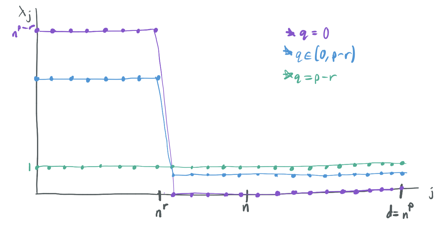
\[\lambda_j = \begin{cases} n^{p - r - q} & j \leq n^r \\ \frac{1 - n^{-q}}{1 - n^{r - p}} & j \geq n^r \end{cases}\]for \(p > 1\), \(r \in (0, 1)\), and \(q \in (0, p-r)\). It’s called a bilevel ensemble because the first \(n^r\) coordinates are drawn from higher variance normal distributions than the remaining \(n^p - n^r\) coordinates. A few notes on this model:
- Because \(p > 1\), \(d = \omega(n)\) and the model is always over-parameterized.
- \(r\) governs the number of high-importance features. Because \(r < 1\), there must always be a sublinear number of high-importance features.
- If \(q\) were permitted to be \(p - r\), then the model would be spherical or isotropic and have \(\lambda_j = 1\) for all \(j\). On the other hand, if \(q = 0\), \(\lambda_j = 0\) for \(j \geq n^r\) and all of the variance would be on the first \(n^r\) features. Thus, \(q\) modulates how much more variance the high-importance features have than the low-importance features.
-
The variances are normalized to have their \(L_1\) norms always be \(d = n^p\):
\[\|\lambda\|_1 = \sum_{j=1}^{n^d} \lambda_j = n^{p} \cdot n^{-q} + \frac{(n^p - n^r)(1 - n^{-q})}{1 - n^{r-p}} = n^{p} \cdot n^{-q} + n^p (1 - n^{-q}) = n^p.\] -
We can compute the effective dimension terms used in the BLLT19 paper:
\[r_k(\Sigma) = \frac{\sum_{j > k} \lambda_j}{\lambda_{k+1}} = \begin{cases} \frac{(n^r - k)n^{p-q} + n^p (1 - n^{-q})}{n^{p-r-q}} &= \Theta(n^{r + q}) & k < n^r \\ n^p - k & & k \geq n^r. \end{cases}\] \[R_k(\Sigma) = \frac{\left(\sum_{j > k} \lambda_j\right)^2}{\sum_{j > k} \lambda_j^2}= \begin{cases} \Theta(\min(n^p, n^{r + 2q})) & k < n^r \\ n^p - k & k \geq n^r. \end{cases}\]
The labels \(y\) are chosen with the 1-sparse linear model, which only considers one of the coordinates. That is, for some \(t \leq n^r\), we let \(w^* = \lambda_t^{-1/2} e_t\), where \(e_t \in \mathbb{R}^d\) is the vector that is all zeroes, except for a one at index \(t\). Note that \(\|w^*\|^2 = \lambda_t^{-1} = n^{r+q - p}\). That is, the labels are \(\text{sign}(\langle w^*, x\rangle) = \text{sign}(x_t)\). (For regression, we instead think of the labels as \(\langle w^*, x\rangle = \lambda_t^{-1/2} x_t\).)
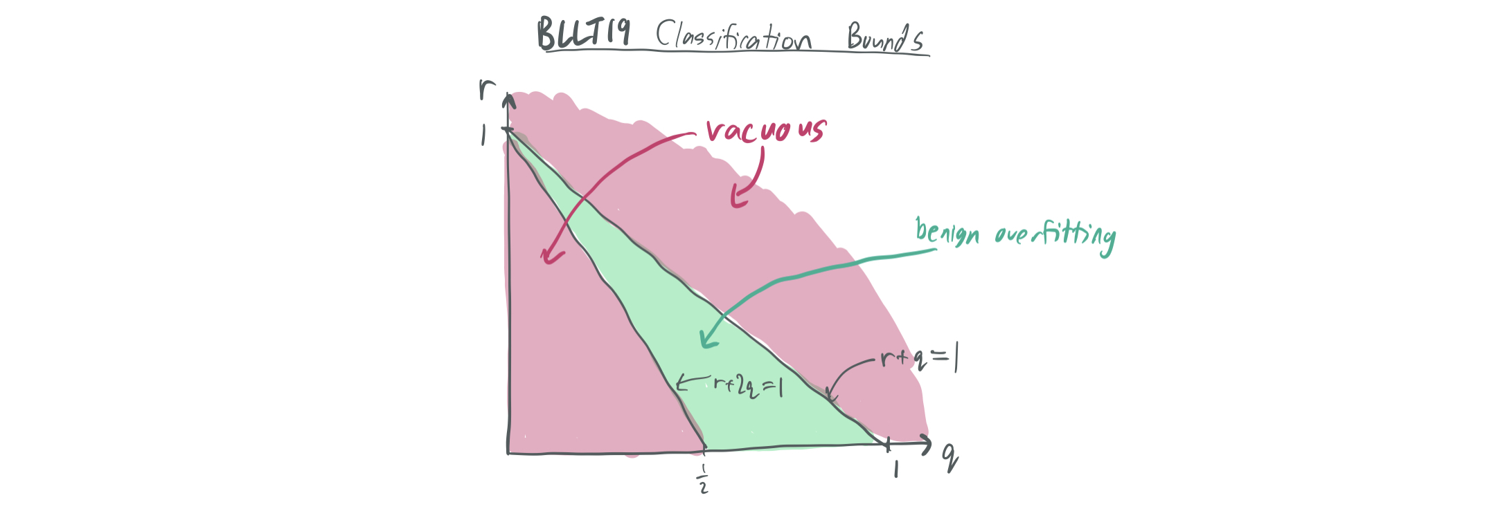
From this data model alone, we can plug in the bounds of BLLT19 to see what they tell us. Note: There actually isn’t a perfect analogue here, because BLLT includes additive label noise with variance \(\sigma^2\), while this blog post only considers the noiseless case of MNSBHS20. The purpose of these bounds is to illustrate what is known about a similar model.
- If \(r + q > 1\), then \(k^* = \min\{k \geq 0: r_k(\Sigma) = \Omega(n)\}\) is roughly \(n^p - O(n)\), which means that the \(\frac{k^*}{n}\) term of the bound makes the bound vacuous.
-
If \(r + q < 1\), then \(k^* = 0\). Then, the BLLT19 bounds yield an excess risk of at most
\[O\left( \|w^*\|^2 \lambda_1 \sqrt{\frac{r_0(\Sigma)}{n}} + \frac{\sigma^2 n}{R_{0}(\Sigma)} \right) = O\left( \sqrt{n^{r + q - 1}}+ \sigma^2 \max(n^{1-p}, n^{1-r-2q}) \right).\]For this bound to trend towards zero, it must be true that \(r + 2q > 1\) and that \(r+ q < 1\), which is already guaranteed.
The bound given in the paper at hand will look slightly different. (e.g. it won’t have the first requirement because noise is done differently.) In addition, it will distinguish between benign overfitting in the classification and regression regimes and show that it’s easier to obtain favorable generalization error bounds for regression.
Main results
They have two types of main results: Theorem 1 shows the sufficient conditions for the coincidence of the SVM and OLS weights \(w_{SVM}\) and \(w_{OLS}\), and Theorem 2 analyzes the generalization of the excess errors of both classification and regression.
When does SVM = OLS?
Theorem 1: For sufficiently large \(n\), \(w_{SVM} = w_{OLS}\) with high probability if
\(\|\lambda\|_1 = \Omega(\|\lambda\|_2 n \sqrt{\log n} + \|\lambda\|_\infty n^{3/2} \log n)\).
Equivalently, it must hold that \(R_0(\Sigma) = \Omega(\sqrt{n}(\log n)^{1/4})\) and \(r_0(\Sigma) = \Omega(n^{3/2} \log n)\). The holds for the bilevel model when \(r + q > \frac{3}{2}\).
In the two follow-ups, this bound is changed to \(r_0(\Sigma) = \Omega(n \log n)\) and the phenomenon is shown to NOT occur when \(R_0(\Sigma) = O(n \log n)\). Thus, this can actually be shown to occur for the bilevel model when \(r + q > 1\).
The proof of the theorem in this paper relies on applying bounds on Gaussian concentration and properties of the inverse-Wishart distribution. The future results rely on tighter concentration bounds, a leave-one-out equivalence that is true when a sample is a support vector, and a trick that relates the relevant quantities to a collection of independent random variables.
Generalization bounds
Their generalization bounds apply to the OLS solutions for two cases, (1) where the labels are real-valued and (2) where the labels are Boolean \(\{-1,1\}\). We call the minimum norm solutions of these \(w_{OLS, real}\) and \(w_{OLS, bool}\). Thus, when \(r\) and \(q\) are large enough for Theorem 1 to guarantee that OLS = SVM, then the bounds for Boolean labels apply.
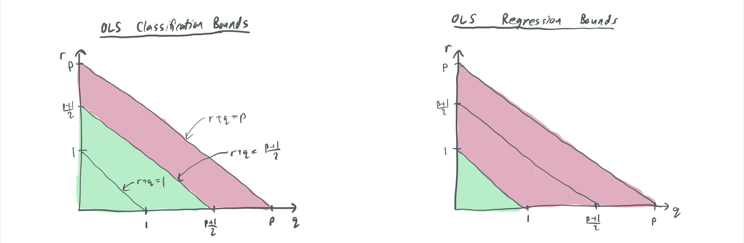
Theorem 2: For a bilevel data model that is 1-sparse without label noise, the classification error \(\lim_{n \to \infty} \mathrm{Pr}[\langle x, w_{OLS, bool}\rangle\langle x, w^*\rangle > 0]\) and regression excess MSE error \(\lim_{n \to \infty} \mathbb{E}[\langle x, w^* - w_{OLS, real} \rangle^2]\) satisfy the following for the given settings of \(p\), \(q\), and \(r\):
| Classification error \(w_{OLS, bool}\) | Regression error \(w_{OLS, real}\) | |
| \(r + q \in (0, 1)\) | 0 | 0 |
| \(r + q \in (1, \frac{p+1}{2})\) | 0 | 1 |
| \(r + q \in (\frac{p+1}{2}, p)\) | 1 | \(\frac12\) |
This table tells us several things about the differences in generalization between classification and regression.
- When \(\Sigma\) has a relatively even distribution of variance between the high-importance and low-importance coordinates and when there are relatively few coordinates, there tends to be favorable generalization for both classification and regression. The reverse is true when there is a sharp cut-off between variances and when there are many high-importance features. This fits a similar intuition to BLLT19, which forbids too sharp a decay of variances.
- One might observe that this doesn’t have the other requirement from BLLT: that the variances do not decay too gradually, which is enforced by \(r + 2q > 1\). This is absent here because this data model does not include label noise, so the risk of a model being corrupted by overfitting noisy labels is minimized.
- There is also a regime in between where classification generalizes well, but regression does not.
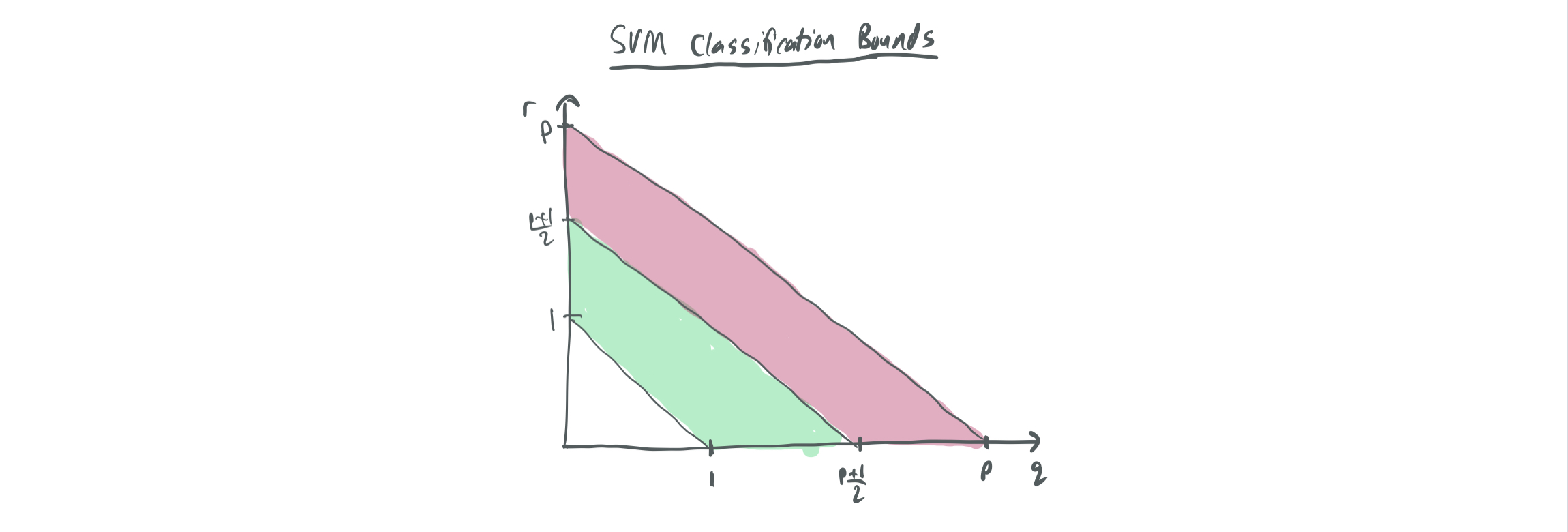
By combining the improved results on support vector proliferation with Theorem 2, we can obtain the following table of results for SVM vs OLS.
| Classification error \(w_{SVM}\) | Regression error \(w_{OLS, real}\) | |
| \(r + q \in (1, \frac{p+1}{2})\) | 0 | 1 |
| \(r + q \in (\frac{p+1}{2}, p)\) | 1 | \(\frac12\) |
How do these generalization bounds work? They’re similar to the flavor of argument given in MVSS19, which considers signal bleed and signal contamination. Put roughly, an interpolating model can perform poorly if either the true signal gets split up among a bunch of orthogonal aliases that each interpolate the training data (signal bleed), or too many spurious correlations are incorporated into the chosen alias (signal contamination). They assess and bound these notions by introducing the survival and contamination terms as
\[\mathsf{SU}(w, t) = \frac{w_t}{w^*_t} = \sqrt{\lambda_t} w_t \ \text{and} \ \mathsf{CN}(w, t) = \sqrt{\mathbb{E}[(\sum_{j\neq t} w_j x_j)^2]} = \sqrt{\sum_{j \neq t} \lambda_j w_j^2}\]This formulation is easy due to the 1-stable assumption of the labels. It seems like it may be possible to write something similar without this data model, but it would probably require much uglier expressions and more complex distributional assumptions to make the proof work.
The proof then uses Proposition 1 to relate the classification and regression errors to the survival and contamination terms and concludes by using Lemmas 11, 12, 13, 14, and 15 to place upper and lower bounds on those terms. Prop 1 shows the following relationships:
\[\mathrm{Pr}[\langle x, w_{OLS, bool}\rangle\langle x, w^*\rangle > 0] = \frac12 - \frac1{\pi} \tan^{-1} \left(\frac{\mathsf{SU}(w, t)}{\mathsf{CN}(w, t)} \right)\] \[\mathbb{E}[\langle x, w^* - w_{OLS, real} \rangle^2] = (1 - \mathsf{SU}(w, t))^2 + \mathsf{CN}(w, t)^2\]From looking at these terms, it should be intuitive why classification error is more likely to go to zero than regression error: It is sufficient for \(\mathsf{CN}(w, t)\) to become arbitrarily small for the the classification error to approach zero, even if \(\mathsf{SU}(w, t)\) is a constant smaller than 1. On the other hand, it must be the case that \(\mathsf{CN}(w, t)\to 0\) and \(\mathsf{SU}(w, t)\to 1\) for the regression error to go to zero.
The concentration bounds in the lemmas are gory and I don’t plan to go into them here. They rely on a slew of concentration bounds that are made possible by the Gaussianity of the inputs and the tight control of their variances.
Closing thoughts
This was another really interesting paper for me, although I wasn’t quite brave enough to venture through all of the proofs of this one. It’s primarily interesting as a proof of concept; the assumptions are prohibitively restrictive (only one relevant coordinate, Gaussian inputs), but the proofs would have been sickening to the point of being unreadable if many of these assumptions were dropped. This paper was an inspiration for my collaborators and me to investigate support vector proliferation in more depth, and these are a nice complement to CL20, which proves bounds for more restricted values of \(d\) and without relying on limits.
Thanks for joining me once again! The next entry–and possibly the last entry of this series–will be posted next week. When the actual exam occurs in two weeks, I might have one last recap post of what’s been discussed so far.
Comments